Table of Contents
- Images and digital spaces
- Creating (unsigned) cells in a cellular grid space
- Cells may be unsigned or signed
- Accessing and modifying cell coordinates.
- Moving within the cellular grid space
- Cell topology and directions
- Cell adjacency and neighborhood
- Cell incidence
- Periodic Khalimsky space and per-dimension closure specification.
- Unbounded cellular grid space
- Author(s) of this documentation:
- by Jacques-Olivier Lachaud, Bertrand Kerautret and Roland Denis
Part of the Topology package.
This part of the manual describes how to define cellular grid space or cartesian cubic spaces, as well as the main objects living in these spaces. A lot of the ideas, concepts, algorithms, documentation and code is a backport from ImaGene.
Images and digital spaces
2D images are often seen as two dimensional arrays, where each cell is a pixel with some value (a gray level, a color). If \(\mathbf{Z}\) is the set of integer numbers, then an image is a map from a rectangular subset of \(\mathbf{Z} \times \mathbf{Z}\) to some space (gray levels, colors).
More generally, a nD image is a map from a parallelepipedic subset of \(\mathbf{Z}^n\) to some space (gray levels, colors).
Many algorithms need to represent positions in images (ie pixels and voxels), in order to represent regions in images. Often, we need also to measure the shape of a region, for instance its perimeter, or we may be interested in the interface between two regions. In these cases, it is often convenient (and generally it is also the theoretic way) to represent other elements in digital spaces, such as paths in-between regions, the thin boundary or surface of a region, etc. We need in this case to represent not only the "squares" (pixels) or "cubes" (voxels) of images, but also their faces, edges, vertices.
We therefore model not only n-dimensional cells (the hypercubes in nD), but also all the lower dimensional cells of the space. For instance, in 2D, we have:
- 2-dimensional cells (closed unit square) = pixels
- 1-dimensional cells (closed unit segment) = linels
- 0-dimensional cells (closed point) = pointels
The set of all cells \(\mathbf{F}^n\) is called the n-dimensional space of cubical complexes, or n-dimensional cellular grid space. The couple \((\mathbf{F}^n,\subseteq)\) is a partially ordered set or poset. Let \(X\) be any subset of \(\mathbf{F}^n\). The set \(\mathcal{U}=\{U \subseteq X / \forall x \in U, x^{\uparrow} \subseteq U \}\), where \(x^{\uparrow}=\{y \in X, x \le y\}\) or the up incident cells of x, is a topology on \(X\), called the Aleksandrov topology. Therefore we can use standard combinatorial topology results for any subset of the cellular grid space.
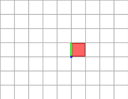
Cells of the cellular grid space are illustrated below. The paving mode of digital space gives a nice illustration of what is this space. The 2-cell is in red, the 1-cell in green, the 0-cell in blue.
Cells in the cubical grid and Khalimsky coordinates
We use now the regularity of the cubical grid to represent it efficiently. In 1D, the cubical grid is a simple line alternating closed points {k} and open unit segments (k,k+1). Khalimsky noticed that this (topological) space is homeomorphic to the integer set \(\mathbf{Z}\), if we declare every even integer as closed and every odd integer as open.
A digital cell in 1D is thus just an integer. Its topology is defined by its parity. The cell 2k is the closed point {k}; the cell 2k+1 is the segment (k,k+1) (considered open).
In 2D, we use the fact that \(\mathbf{Z}^2\) is a cartesian product. A digital cell in 2D is thus a couple of integer
- (2i, 2j): a pointel which is the point set {(i,j)} in the plane
- (2i+1, 2j): an horizontal linel which is the open segment {(i,i+1) x j} in the plane.
- (2i, 2j+1): a vertical linel which is the open segment {i x (j,j+1)} in the plane.
- (2i+1, 2j+1): a pixel which is the open square {(i,i+1) x (j,j+1)} in the plane.
In nD, the principle is the same. A cell is thus uniquely identified by an n-tuple of integers whose parities define the topology of the cell. These integers are called the Khalimsky coordinates of the cell.
For instance, the pixel (x,y) of the digital space \(\mathbf{Z}^2\) corresponds to the 2-cell (2x+1,2y+1) of the cellular grid space \(\mathbf{F}^2\).
Models for cellular grid spaces
Instead of choosing a specific implementation of a cellular grid space, we keep the genericity and efficiency objective of DGtal by defining a cellular grid space as the concept CCellularGridSpaceND. It provides a set of types (Cell, SCell, etc) and methods to manipulate cells of arbitrary dimension. Models of CCellularGridSpaceND are:
- the KhalimskySpaceND template class, that allows per-dimension closure specification (open, closed or periodic).
- the — yet to come — CodedKhalimskySpaceND class, a backport from class KnSpace of ImaGene.
The inner types are:
- Integer: the type for representing a coordinate or component in this space.
- Size: the type for representing a size (unsigned)
- Cell: the type of unsigned cells
- SCell: the type of signed cells
- Sign: the sign type for cells
- DirIterator: the type for iterating over directions of a cell
- Point: the type for representing a digital point in this space
- Vector: the type for representing a digital vector in this space
- Space: the associated digital space type
- CellularGridSpace: this cellular grid space
- Cells: a sequence of unsigned cells
- SCells: a sequence of signed cells
- CellSet: a set container that stores unsigned cells (efficient for queries like
find, model of boost::UniqueAssociativeContainer and boost::SimpleAssociativeContainer). - SCellSet: a set container that stores signed cells (efficient for queries like
find, model of boost::UniqueAssociativeContainer and boost::SimpleAssociativeContainer). - SurfetSet: a set container that stores surfels, i.e. signed n-1-cells (efficient for queries like
find, model of boost::UniqueAssociativeContainer and boost::SimpleAssociativeContainer). - CellMap<Value>: an associative container Cell->Value rebinder type (efficient for key queries). Use as
typenameX::template CellMap<Value>::Type, which is a model of boost::UniqueAssociativeContainer and boost::PairAssociativeContainer. - SCellMap<Value>: an associative container SCell->Value rebinder type (efficient for key queries). Use as
typenameX::template SCellMap<Value>::Type, which is a model of boost::UniqueAssociativeContainer and boost::PairAssociativeContainer. - SurfelMap<Value>: an associative container Surfel->Value rebinder type (efficient for key queries). Use as
typenameX::template SurfelMap<Value>::Type, which is a model of boost::UniqueAssociativeContainer and boost::PairAssociativeContainer.
Methods include:
- Cell creation services
- Read accessors to cells
- Write accessors to cells
- Conversion signed/unsigned cells
- Cell topology services
- Direction iterator services for cells
- Unsigned cell geometry services
- Signed cell geometry services
- Neighborhood services
- Incidence services
- Interface
An comprehensive description is given in CCellularGridSpaceND.
Creating a cellular grid space
We use hereafter the model KhalimskySpaceND. To create a 2D cellular grid space where cells have coordinates coded with standard int (32 bits generally), we can write:
Note that the cellular grid space is limited by the given bounds. Since the user has chosen a closed space, the Khalimsky coordinates of cells are bounded by:
- lower bound: (-3*2, -4*2)
- upper bound: (5*2+2, 3*2+2)
Another frequent way of constructing a cellular grid space is to start from a preexisting digital space and HyperRectDomain. You can define the associated cellular grid space as follows:
If you wish to build a digital space and a HyperRectDomain from a cellular grid space K, you may write:
Last but not least, for standard users it is generally enough to use the default types provided in DGtal/helpers/StdDefs.h.
Creating (unsigned) cells in a cellular grid space
There are many ways of creating cells within a cellular grid space. The simplest way is certainly to give the Khalimsky coordinates of the cell you wish to create. Its topology is then induced by its coordinates. We use generally KhalimskySpaceND::uCell for arbitrary cells, KhalimskySpaceND::uSpel for n-dimensional cells, KhalimskySpaceND::uPointel for 0-dimensional cells.
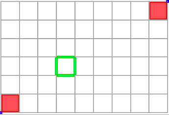
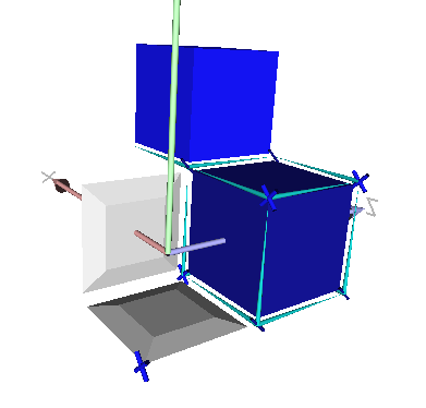
The full code of this example is in file ctopo-1.cpp. Pointels or 0-cells are displayed in blue, linels or 1-cells in green, pixels or 2-cells in red. Note that KhalimskySpaceND::uCell requires Khalimsky coordinates while the two others require digital coordinates (the topology is known in the two latter cases).
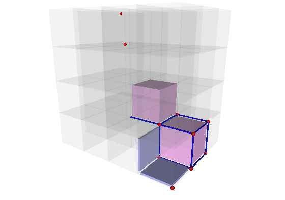
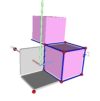
The file ctopo-1-3d.cpp shows another example in 3D:
Cells may be unsigned or signed
Up to now, we have only consider unsigned cells (type Cell). However it is often convenient to assign a sign (POS or NEG) to a cell, a kind of orientation. The sign is especially useful to define boundary operators and digital surfaces. It is also used in algebraic topological models of cubical complexes, for instance to define chains (formal sums of cells).
Signed cells have type SCell. They are created using methods KhalimskySpaceND::sCell for arbitrary cells, KhalimskySpaceND::sSpel for n-dimensional cells, KhalimskySpaceND::sPointel for 0-dimensional cells. The user gives the sign at creation, either K.POS or K.NEG if K is the space.
You may use methods KhalimskySpaceND::sSign, KhalimskySpaceND::sSetSign KhalimskySpaceND::signs, KhalimskySpaceND::unsigns, KhalimskySpaceND::sOpp, respectively to get the sign of a signed cell, to change the sign of a signed cell, to sign an unsigned cell, to unsign a signed cell, and to compute the cell with opposite sign.
All methods concerning unsigned cells are prefixed by u, all methods concerning signed cells are prefixed by s.
Note that the sign of the signed and unsigned are well taken into account in the display with DGtal::PolyscopeViewer .
Accessing and modifying cell coordinates.
Since one does not necessarily know which model of CCellularGridSpaceND you may be using, you cannot access the cell coordinates directly. Therefore a model of CCellularGridSpaceND provides a set of methods to access and modify cell coordinates and topology. Here a few of them (with the model example KhalimskySpaceND)
- Read accessors to coordinate(s)
- KhalimskySpaceND::uKCoord, KhalimskySpaceND::sKCoord (read Khalimsky coordinate)
- KhalimskySpaceND::uCoord, KhalimskySpaceND::sCoord (read digital coordinate)
- KhalimskySpaceND::uKCoords, KhalimskySpaceND::sKCoords (read Khalimsky coordinates)
- KhalimskySpaceND::uCoords, KhalimskySpaceND::sCoords (read digital coordinates)
- Write accessors to coordinate(s)
- KhalimskySpaceND::uSetKCoord, KhalimskySpaceND::sSetKCoord (write Khalimsky coordinate)
- KhalimskySpaceND::uSetCoord, KhalimskySpaceND::sSetCoord (write digital coordinate)
- KhalimskySpaceND::uSetKCoords, KhalimskySpaceND::sSetKCoords (write Khalimsky coordinates)
- KhalimskySpaceND::uSetCoords, KhalimskySpaceND::sSetCoords (write digital coordinates)
Moving within the cellular grid space
Note that you dispose also of a whole set of methods to determine cells according to different geometric queries. The following methods do not change the topology of the input cell only the coordinates. Again the prefix u is related to method taking as input unsigned cells while the prefix s is related to signed cells:
- Getting the first or last cell of the space: KhalimskySpaceND::uFirst, KhalimskySpaceND::uLast, KhalimskySpaceND::sFirst, KhalimskySpaceND::sLast
- Moving to the adjacent cell with one coordinate greater or one coordinate lower: KhalimskySpaceND::uGetIncr, KhalimskySpaceND::uGetDecr, KhalimskySpaceND::sGetIncr, KhalimskySpaceND::sGetDecr, or moving to an arbitrary cell along some axis with KhalimskySpaceND::uGetAdd and KhalimskySpaceND::uGetSub, KhalimskySpaceND::sGetAdd and KhalimskySpaceND::sGetSub.
- Testing whether you are the cell with maximal or minimal coordinate along some axis with KhalimskySpaceND::uIsMax or KhalimskySpaceND::uIsMin, KhalimskySpaceND::sIsMax or KhalimskySpaceND::sIsMin
- Getting the cell along some axis that has same coordinates as the input cell but for one which belongs the minimal or maximal accepted in this space: KhalimskySpaceND::uGetMax and KhalimskySpaceND::uGetMin, KhalimskySpaceND::sGetMax and KhalimskySpaceND::sGetMin
- Project a cell along some coordinate onto the axis-aligned hyperplanes spanned by a cell with KhalimskySpaceND::uProject and KhalimskySpaceND::uProjection, KhalimskySpaceND::sProject and KhalimskySpaceND::sProjection
- Computes the distance of the cell to the bounds of the space along some axis with KhalimskySpaceND::uDistanceToMax and KhalimskySpaceND::uDistanceToMin, KhalimskySpaceND::sDistanceToMax and KhalimskySpaceND::sDistanceToMin
Getting the next cell in this space such that if one starts from the first cell (with same topology) of the space and iterates this process, then all cells of the space with same topology were visited. This may be done with KhalimskySpaceND::uNext, KhalimskySpaceND::sNext. Below is a code snippet that does a scanning of all cells of same topology between first and last cell.
Cell first, last; // lower and upper boundsCell p = first;do{ // ... whatever [p] is the current cell}while ( K.uNext( p, first, last ) );For instance (see. khalimskySpaceScanner.cpp) you will obtain the default following scan:
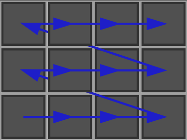
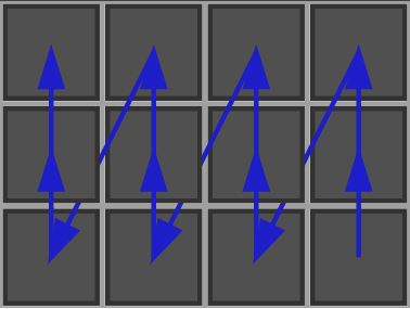
- The scan can also be done by explicitly controlling the order: You will obtain the following scan:
- Translating arbitrarily a cell in the space with KhalimskySpaceND::uTranslation and KhalimskySpaceND::sTranslation.
Cell topology and directions
As said above, the cell topology is defined by the parity of its Khalimsky coordinates. The number of coordinates where the cell is open define the dimension of the cell. A cell of maximal dimension (n) is called a pixel in 2D, a voxel in 3D, and sometimes called a spel or xel in nD. A cell of minimal dimension (0) is often called a pointel. n-1 cells are called surfels (or sometimes linels in 2D). Here are the methods related to the cell topology.
- the dimension of a cell is given by KhalimskySpaceND::uDim and KhalimskySpaceND::sDim.
- whether a cell is open or not along some axis is returned by KhalimskySpaceND::uIsOpen and KhalimskySpaceND::sIsOpen.
- whether a cell is a surfel or not is returned by KhalimskySpaceND::uIsSurfel and KhalimskySpaceND::sIsSurfel. NB: you should use it instead of comparing the dimension of the cell with n-1, depending on the model of cellular grid space chosen.
- the integer coding the topology of the cell such that the k-th bit is 1 whenever the cell is open along the k-th axis is returned by KhalimskySpaceND::uTopology and KhalimskySpaceND::sTopology.
you may iterate over all open coordinates (or all closed coordinates) of a cell with the iterator returned by KhalimskySpaceND::uDirs and KhalimskySpaceND::sDirs (KhalimskySpaceND::uOrthDirs and KhalimskySpaceND::sOrthDirs for closed coordinates), such as in this snippet:
KSpace::Cell p;...for ( KSpace::DirIterator q = ks.uDirs( p ); q != 0; ++q ){Dimension dir = *q;...}typename PreCellularGridSpace::DirIterator DirIteratorDefinition KhalimskySpaceND.h:422
Cell adjacency and neighborhood
You may obtain the cells of same topology which are (face-)adjacent to a given cell with the following methods:
- the neighborhood of a given cell within the space are given by KhalimskySpaceND::uNeighborhood and KhalimskySpaceND::sNeighborhood, while the proper neighborhood is returned by KhalimskySpaceND::uProperNeighborhood and KhalimskySpaceND::sProperNeighborhood.
- the cell that is adjacent forward or backward along some given axis is returned by KhalimskySpaceND::uAdjacent and KhalimskySpaceND::sAdjacent.
Cell incidence
Cells incident to some cell touch the cell but do not have the same dimension. Cells lower incident to a cell have lower dimensions, cells upper incident to a cell have higher dimensions. Specific rules determine the sign of incident cells to a signed cell:
- A first rule is that along some axis, the forward and the backward incident cell have opposite sign.
- A second rule is that the rules are invariant by translation of cells.
- A third rule is that changing the sign of the cell changes the sign of all incident cells.
- A last rule is that taking an incident cell along some axis k then taking an incident cell along some other axis l will give a cell that has the opposite sign as if the incidence was taken before along l and after along k.
These rules together allow the definition of (co)boundary operators, which are homomorphisms between chains of cells. They have the property that applied twice they give the null chain. Otherwise said, the boundary of a set of cells has an empty boundary.
The cell incident to some given cell along some axis and in forward or backward direction is returned by KhalimskySpaceND::uIncident and KhalimskySpaceND::sIncident.
// ptld and ptdl have opposite signs.Represents a signed cell in a cellular grid space by its Khalimsky coordinates and a boolean value.Definition KhalimskySpaceND.h:209- The set of cells low incident to a given cell (i.e. just 1 dimension less) is returned by KhalimskySpaceND::uLowerIncident and KhalimskySpaceND::sLowerIncident.
- The set of cells up incident to a given cell (i.e. just 1 dimension more) is returned by KhalimskySpaceND::uUpperIncident and KhalimskySpaceND::sUpperIncident.
- The proper faces of an unsigned cell are returned by KhalimskySpaceND::uFaces.
- The proper cofaces of an unsigned cell are returned by KhalimskySpaceND::uCoFaces.
One of the two cells that are incident to some signed cells along some axis has a positive sign. The orientation (forward or backward) is called the direct orientation. It is returned by KhalimskySpaceND::sDirect. It is worth to note that the following assertion is always true:
- You may obtain straightforwardly the positive incident cell along some axis with KhalimskySpaceND::sDirectIncident and the negative incident cell along some axis with KhalimskySpaceND::sIndirectIncident.
Periodic Khalimsky space and per-dimension closure specification.
In addition to the CCellularGridSpaceND requirements, KhalimskySpaceND allows the use of different closures for each dimension and the use of periodic dimension.
The closure is specified at the space initialization:
Therefore, any coordinates are valid along a periodic dimension but the coordinates accessors of KhalimskySpaceND will always return a coordinate between the two bounds given at the initialization:
It is also possible to span a sub-space that crosses the bounds along a periodic dimension:
Unbounded cellular grid space
If you need to arbitrarily manipulate the cells coordinates without bounds checking, or if you simply doesn't need a bounded space, you may consider KhalimskyPreSpaceND.
It is a model of CPreCellularGridSpaceND, that is a base concept of CCellularGridSpaceND. The main difference is that CPreCellularGridSpaceND doesn't require to initialize the space with bounds and some bounds related methods (like KhalimskySpaceND::uGetMin) are not available.
Therefore, KhalimskyPreSpaceND is a purely static class that provides almost all the methods of KhalimskySpaceND but without bounds influence (coordinates validity, restricted neighborhood, ...) and is also fully compatible with KhalimskySpaceND-based algorithms when bounds are not necessary.
The main features are:
- direct manipulation of the Khalimsky coordinates through the
coordinatespublic member of KhalimskyPreCell and SignedKhalimskyPreCell:using KPreSpace = DGtal::KhalimskyPreSpaceND<2, int>;KPreSpace::Cell a = KPreSpace::uSpel( {1, 1} );KPreSpace::SCell b = KPreSpace::sPointel( {12, 5}, true );const auto pt_diff = b.coordinates - a.coordinates;a.coordinates[0] += 2;Aim: This class is a model of CPreCellularGridSpaceND. It represents the cubical grid as a cell compl...Definition KhalimskyPreSpaceND.h:379 - direct construction of a pre-cell from its Khalimsky coordinates: KPreSpace::Cell precell( Point( 4, 5 ) ); // OK// KSpace::Cell cell( Point( 4, 5 ) ); // Compilation error.// Cell creation is only possible through a valid KhalimskySpaceND.
- easy conversion from a cell to a pre-cell using the KhalimskyCell::preCell and SignedKhalimskyCell::preCell methods, or using the implicit conversion: KSpace::Cell cell = K.uSpel( {1, 1} );// KSpace::PreCell is an alias to DGtal::KhalimskyPreCell<2, int>KSpace::PreCell preA = cell; // implicit conversion to a pre-cell.KSpace::PreCell preB = cell.preCell(); // explicit conversion to a pre-cell using KhalimskyCell::preCell./* Implicit conversion when calling function acceptinga pre-cell as parameter is possible as long as template deductionis not needed on the pre-cell template parameters./myAlgorithmThatWorksOnPreCell( cell );PreCell const & preCell() constReturns the underlying constant pre-cell.
- most KhalimskySpaceND methods exist in KhalimskyPreSpaceND (take a look to the KhalimskyPreSpaceND documentation or just to the difference between CCellularGridSpaceND and CPreCellularGridSpaceND).
- Conversion from a pre-cell to a cell needs the associate Khalimsky space in order to ensure that the coordinates are valid: using KPreSpace = DGtal::KhalimskyPreSpaceND<2, int>;KPreSpace::Cell preA = KPreSpace::uSpel( {1, 1} );KPreSpace::SCell preB = KPreSpace::sPointel( {12, 5}, true );// KSpace::Cell cell = preA; // <- doesn't compile.KSpace::SCell cell2 = K.sCell( preB ); // Will failed at runtime (in DEBUG mode) because preB is outside K.