Table of Contents
- Author(s) of this documentation:
- Caissard Thomas
Continuous Laplace–Beltrami operator
Let \(M\) be a smooth manifold. The linear operator \(\Delta : C^2(\partial M) \rightarrow C^2(\partial M)\) (where \(C^2(\partial M)\) is the set of twice differentiable function acting on \(\partial M\)) defined by
\[ \Delta u = \nabla^2 u = \nabla \cdot \nabla u, \]
is called the Laplace–Beltrami operator.
- Note
- The sign of the operator is arbitrary, and one may found in the literature the alternative definition \(-\nabla \cdot \nabla u\) for \(\Delta u\).
For example, in \( \mathbb{R}^d \), the operator is the sum of the second derivatives:
\[ \Delta_{\mathbb{R}^d} u(x) = \sum_i \frac{\partial^2}{\partial x_i^2}u(x). \]
This operator can be expressed in local coordinates system on a manifold given the metric tensor \(g_{ij}\):
\[ \Delta u = \frac{1}{\sqrt{g}} \partial_i \left( \sqrt{|g|}g^{ij}\partial_j u \right), \]
with the Einstein notation implied (meaning that repeated indexes are summed over), \( \sqrt{|g|}\) is the absolute value of the determinant of \( g_{ij} \) and \( \partial_i = \frac{\partial}{\partial x^i}\) is the basis of the tangent plane \(T_p M\) at a point \(p\).
The operator can also be written in a coordinate-free manner using the exterior calculus theory. Given a function \(w\) (ie. a 0-form) we have
\[ \Delta w = \star d \star d w, \]
where \(\star\) is the hodge operator and \( d \) the exterior derivative.
The Laplace–Beltrami operator from the Heat Equation
Let \(g : \partial M \times (0, T) \rightarrow \mathbb{R}\) be a time-dependent function which solves the partial differential equation called the heat equation:
\[ \Delta g(x, t) = \frac{\partial}{\partial t}g(x, t), \]
with initial condition \(u = g(\cdot, 0) : \partial M \rightarrow \mathbb{R}\) which is the initial temperature distribution.
An exact solution is:
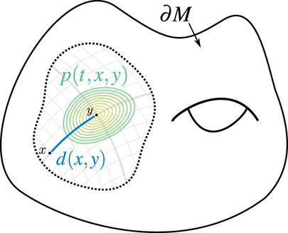
\[ \int_{y\in \partial M} p(t, x, y) u(y) dy, \]
where \(p \in C^\infty(\mathbb{R}^+ \times \partial M \times \partial M)\) is the heat kernel [105].
There is a wide range of studies on the behavior of \(p\) when \(t\) tends to zero (called small time asymptotics of diffusion process). Early works include the famous Varadhan formula [121] on closed manifolds with or without borders later extended by Molchanov [96] on a wider class of shapes:
\[ p(t,x,y) \mathrel{\mathop{\sim}\limits_{t \rightarrow 0}} \frac{e^{- \frac{d(x,y)^2}{4 t}}}{(4\pi t)^{\frac{d}{2}}} \]
where \(d(\cdot,\cdot)\) corresponds to the intrinsic geodesic distance. This approximation is not robust in practice and very sensitive to both geodesic distance approximation and numerical errors [41]. Fortunately we know from Belkin et al. [11] that in small time asymptotics, the geodesic distance can be approximated by the \(l_2\) distance:
\[ p(t,x,y) \mathrel{\mathop{\sim}\limits_{t \rightarrow 0}} \tilde{p}(t,x,y) := \frac{e^{ - \frac{||x - y||^2}{4t} }}{(4 \pi t)^{\frac{d}{2}}}, \]
which leads to the following approximated solution of the heat equation:
\[ g(x,t) = \int_{y \in \partial M} \tilde{p}(t,x,y) u(y)dy. \]
By injecting the approximation into the heat equation we obtain:
\[ \Delta g(x, t) = \frac{\partial}{\partial t} \int_{ y\in \partial M } \tilde{p}(t, x, y) u(y)dy. \]
Using a finite difference on \(t\), and the basic property that the integral of the heat kernel must be one:
\[ \Delta g(x, t) = \lim\limits_{t \rightarrow 0} \frac{1}{t} \int_{y\in \partial M } \tilde{p}(t, x, y) (u(y) - u(x))dy. \]
The Discretization on Digital Surfaces
We adapt the formulation of Belkin et al. on digital surfaces (see [18]). In the continuous heat kernel formulation, the parameter \(t\) must tend to zero. On digital surfaces, we set \(t\) as a function of the grid step \(h\), denoted \(t_h\), that tends to zero as \(h\) tends to zero.
- Note
- Typically the time parameter is set to \(t_h = k \cdot h^{\alpha}\) with \(\alpha\) positive and \(k\) is a constant depending on the input shape.
The discretization on digital surfaces is
\[ (\Delta_{DIGI} \, f)({\mathbf{s}}) := \frac{1}{t_h(4 \pi t_h)^{\frac{d}{2}}} \sum_{\mathbf{r}\in \mathbb{F}^d } e^{- \frac{||\dot{\mathbf{r}} - \dot{\mathbf{s}}||^2}{4t_h}} [f(\dot{{\mathbf{r}}}) - f(\dot{{\mathbf{s}}})]\mu(\mathbf{r}), \]
where \(\mathbb{F}^d\) is the set of elements dimension \(d\) (for example surfels in a 2D surface embedded in 3D), \(\dot{\mathbf{r}}\) (resp. \(\dot{\mathbf{s}}\)) is the centroid of the surfel \(\mathbf{r}\) (resp. \(\mathbf{s}\)), and \(\mu(\mathbf{r})\) is equal to the dot product between an estimated normal and the trivial normal orthogonal to the surfel \(\mathbf{s}\). We typically use the Integral Invariant estimator for normal computation.
Hands on the Operator in DGtal
This section provides an overview on how to use the Heat Laplace in DGtal. The operator is embedded inside the DEC structure of DGtal. The following code comes from the file exampleHeatLaplace.cpp. We demonstrate the usage of the heat operator on a function defined on the unit sphere. The laplace operator in spherical coordinates on the unit sphere is
\[ \Delta = \frac{1}{ \sin^2(\theta) } \frac{\partial^2}{\partial \theta^2} + \frac{1}{\sin(\phi)} \frac{\partial}{\partial \phi}( \sin(\phi) \frac{\partial}{\partial \phi} ) \]
We choose the function \(f(x,y,z) = x^2\). Its Laplacian is then \( \Delta f(r, \theta, \phi) = 2 \cos(\theta)^2 ( 2 \cos(\phi)^2 - \sin(\phi)^2 ) + 2( \sin(\theta)^2 - cos(\theta)^2 ) \).
You must first compute the boundary of the surface, that is here for example the set of surfels of the boundary of the unit sphere.
Then, we need to compute the estimated area of a surfel, i.e. the quantity \( \mu \). We use the Integral Invariant estimator to compute the estimated normals of the surfels (see Integral invariant curvature estimator 2D/3D). We use the same parameter \( \alpha = 1 / 3\) for Integral Invariant and our Laplace–Beltrami estimator.
The DEC structure is initialized using the normal estimator (if no normal estimators is given, the surface area will be one as default, which leads to a poor estimation of the laplace operator)
As we compute the laplace operator on surfels, the input function is represented by a 2-form in the dec structure.
- Note
- The order of the input surfels is not the same as the internal order of DEC. You must use getCellIndex from DEC to retrieve the internal order of a cell.
We can now construct the Laplace operator. It is a DualIdentity of 2-forms, i.e. a linear operator acting on 2-forms represented internally by a sparse matrix. The function heatLaplace of DEC is templated by the duality of the operator. If you want to compute the operator on 0-forms (on points), you must pass PRIMAL as template parameter. We use here the dual operator. The function takes as input the grid size \( h \), the time parameter for the convolution \( t_h \) and a variance multiplier for the integration \( K \).
- Note
- As mentioned earlier, the time parameter is generally set to \( t_h = k \cdot h^\alpha \) where \(k\) is a constant depending on the input shape which roughly corresponds to the size of the Gaussian kernel in the euclidean space (here \(k = 0.1\) for the unit sphere).
The integration is done within the cut locus range: we only sum points which euclidean distance is inferior to \( K \sigma = K \sqrt{2t} \) (where \(\sigma\) is the variance of the Gaussian function). Indeed it is known that almost all the mass under a Gaussian in contained within a few multiples of \( \sigma \) (typically two or three time \(\sigma\)).
Finally, the result is computed with a simple matrix multiplication