Table of Contents
- Author(s) of this documentation:
- Jacques-Olivier Lachaud, Bastien Doignies, David Coeurjolly
- Since
- 1.0
Part of the Tutorials.
This part of the manual describes how to use shortcuts to quickly create shapes and surfaces, to traverse surfaces, to save/load images and shapes, and to analyze their geometry.
The following programs are related to this documentation: shortcuts.cpp, shortcuts-geometry.cpp
- Note
- All rendering are made with Blender.
- See also
- Integral invariant curvature estimator 2D/3D for Integral Invariant estimators.
- Digital Voronoi Covariance Measure and geometry estimation for Voronoi Covariance Measure estimators.
Introduction
To use shortcuts, you must include the following header:
And choose an appropriate Khalimsky space according to the dimension of the object you will be processing.
- See also
- moduleCellularTopology
The general philosophy of the shortcut module is to choose reasonable data structures in order to minimize the number of lines to build frequent digital geometry code. For instance, the following lines build a shape that represents the digitization of an ellipsoid.
As one can see, a Parameters object stores parameter values and can be simply updated by the user with the function operator().
- Note
- Big objects (like images, explicit shapes, explicit surfaces) are always returned or passed as smart pointers (with CountedPtr). Smaller objects (like vectors of scalars, etc) are efficiently passed by value. Hence you never have to take care of their lifetime and you do not need to delete them explicitly.
Short 3D examples
We give below some minimalistic examples to show that shortcuts can save a lot of lines of code. All examples need at least the following lines:
Examples requiring geometric functions (ground-truth or estimation) need the following lines (i.e. functions in SHG3):
Load vol file -> ...
-> noisify -> save as vol file.
-> build main connected digital surface
-> extract 2 isosurfaces -> build mesh -> displays them
The following code extracts iso-surfaces (maybe multiple connected components) in the given gray-scale 3D image and builds meshes, which can be displayed.
- Note
- Iso-surfaces are built by duality from digital surfaces. The output triangulated surfaces share similarities with marching-cubes surfaces, but they are guaranteed to be 2-manifold (closed if the surface does not touch the boundary of the domain).
If you wish to display them with two different colors, you may write:
-> extract 2 triangulated isosurfaces -> save as OBJ
The following code extracts all iso-surfaces in the given gray-scale 3D image and saves them as OBJ file with color information.
-> build main digital surface -> breadth first traversal -> save OBJ with colored distance.
You may choose your traversal order ("Default", "DepthFirst", "BreadthFirst").
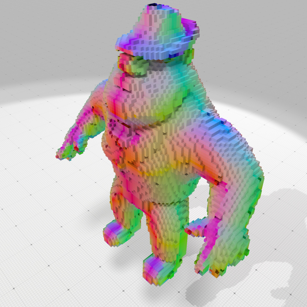
-> build digital surface -> estimate curvatures -> save OBJ.
This example requires ShortcutsGeometry. It shows how tu use the integral invariant curvature estimator on a digital shape model to estimate its mean or Gaussian curvature.
Rendering of Al Capone with estimated mean curvatures (blue is negative, white zero, red is positive, scale is [-0.5, 0.5]). | 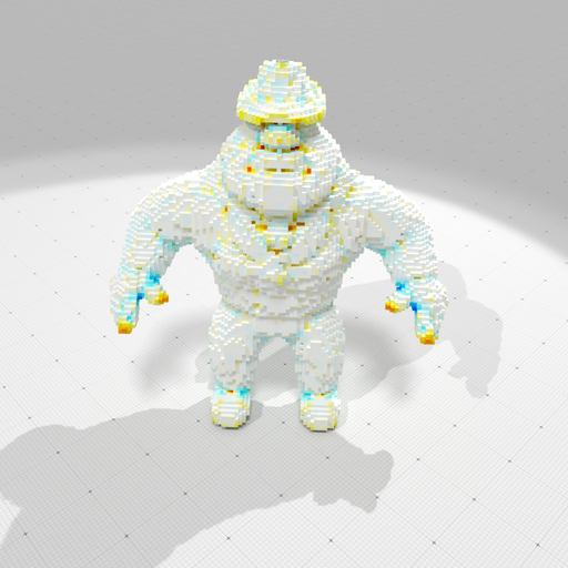
Rendering of Al Capone with estimated Gauss curvatures (blue is negative, white zero, red is positive, scale is [-0.25, 0.25]). |
Build polynomial shape -> digitize -> ...
-> noisify -> save as vol file.
-> build surface -> save primal surface as obj
- Note
- The OBJ file is generally not a combinatorial 2-manifold, since digital surfaces, seen as squares stitched together, are manifold only when they are well-composed.
-> build indexed surface on a subpart
You may choose which part of a domain is digitized as a binary image, here the first orthant is chosen.
-> noisify -> count components -> save OBJ with different colors.
-> extract ground-truth geometry
This example requires ShortcutsGeometry. It shows you how to recover ground-truth positions, normal vectors, mean and Gaussian curvatures onto an implicit 3D shape. For each surfel, the geometry is the one of the point nearest to the given surfel centroid.
-> get pointels -> save projected quadrangulated surface.
This example requires ShortcutsGeometry. It shows you how to get pointels from a digital surface and how to project the digital surface onto the given implicit shape.
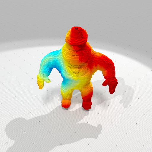
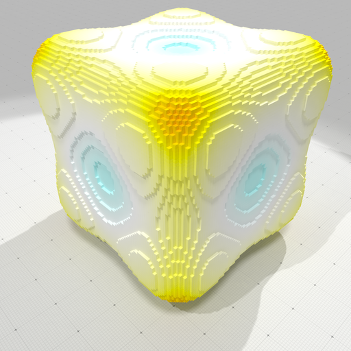
-> extract mean curvature -> save as OBJ with colors
This example requires ShortcutsGeometry. The ground-truth mean curvature is just displayed as a color, using the specified colormap.
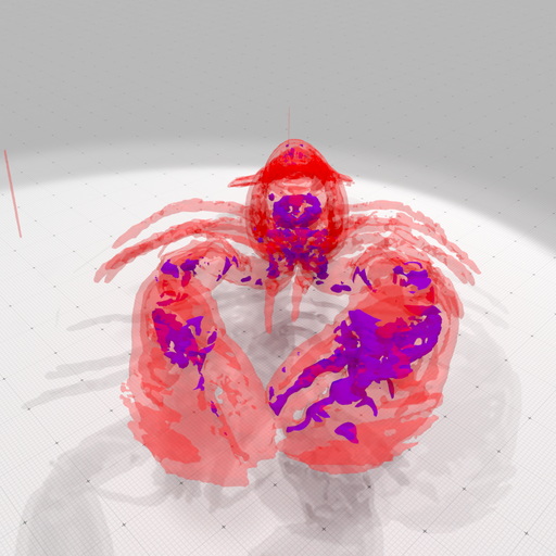
-> extract ground-truth and estimated mean curvature -> display errors in OBJ with colors
This example requires ShortcutsGeometry. Both ground-truth and estimated mean curvature are computed. Then you have functions like ShortcutsGeometry::getScalarsAbsoluteDifference and ShortcutsGeometry::getStatistic to measure errors or ShortcutsGeometry::getVectorsAngleDeviation to compare vectors.
|
Ground truth mean curvature | 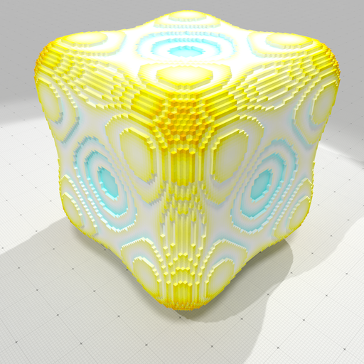
Estimated II mean curvature | 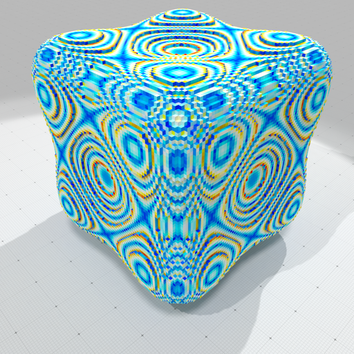
Highlight estimation errors (blue small, red high) |
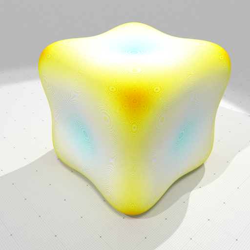
-> build surface -> save primal surface with vcm normals as obj
This example requires ShortcutsGeometry.
- Note
- The OBJ file is generally not a combinatorial 2-manifold, since digital surfaces, seen as squares stitched together, are manifold only when they are well-composed.
|
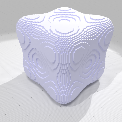
Rendering of goursat-primal.obj (no normals). | 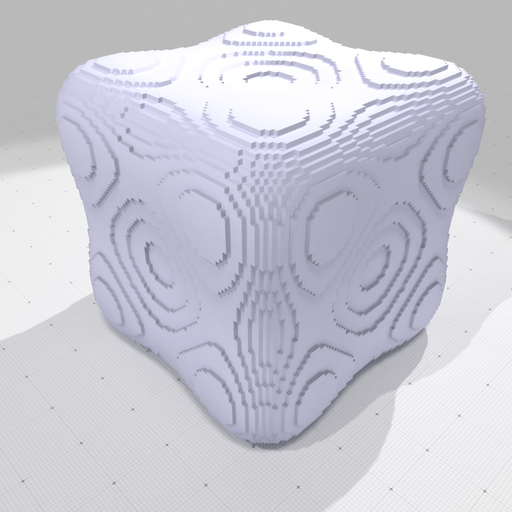
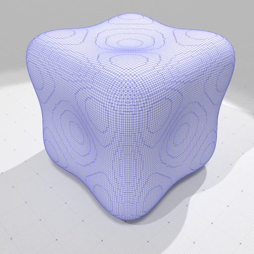
Rendering of goursat-primal-vcm.obj (normals estimated by VCM). Note that staircases effects are still very visible, although normals are good. |
-> digitize implicitly -> estimate II normals and curvature.
This example requires ShortcutsGeometry. You may also analyze the geometry of a digital implicitly defined surface without generating a binary image and only traverse the surface.
-> digitize -> save primal surface and VCM normal field as obj
This example requires ShortcutsGeometry. You may estimate the normals to a surface by the VCM normal estimator.
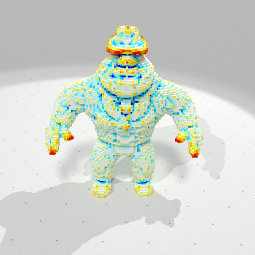
-> digitize -> II normals -> AT piecewise-smooth approximation
This example requires ShortcutsGeometry. You may also use the Ambrosio-Tortorelli functional to get a piecewise smooth approximation of an arbitrary scalar or vector field over a surface. Here we use it to get a piecewise smooth approximation of the II normals.
Piecewise-smooth normals displayed as colors on Al-150 dataset. | 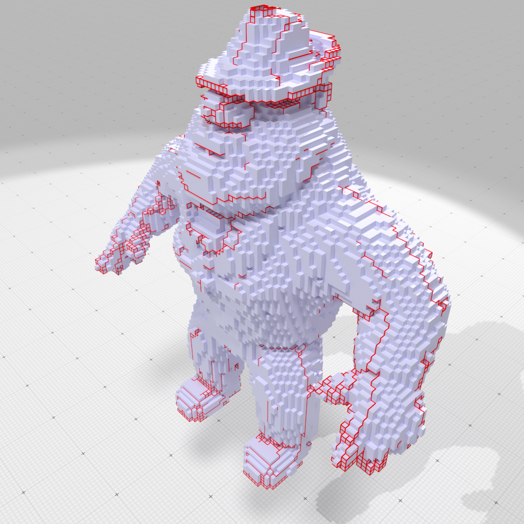
Discontinuities of the piecewise-smooth normal vector field on Al-150 dataset. |
-> load mesh -> CNC curvatures -> export mesh
This example requires ShortcutsGeometry. It shows how tu use the Corrected Normal Current curvature estimator on a mesh model to estimate its mean, Gaussian or principals curvature.
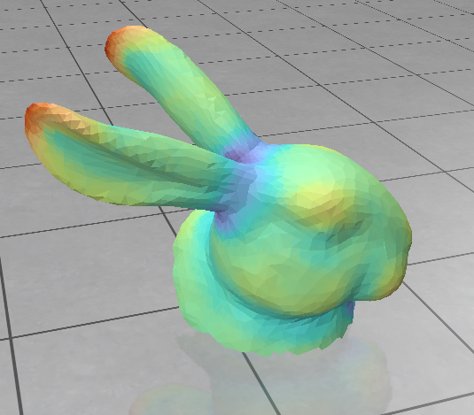
Rendering of Bunny Head with estimated Gauss curvatures | 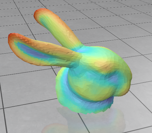
Rendering of Bunny Head with estimated Mean curvatures |
-> digitize -> True principal curvatures
This example requires ShortcutsGeometry. You can easily get the expected principal curvatures and principal directions onto a digitized implicit shape.
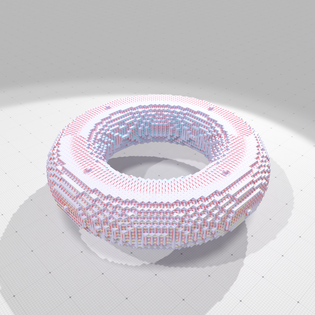
Principal directions of curvatures colored according to their value (blue negative, red positive) on a torus. | 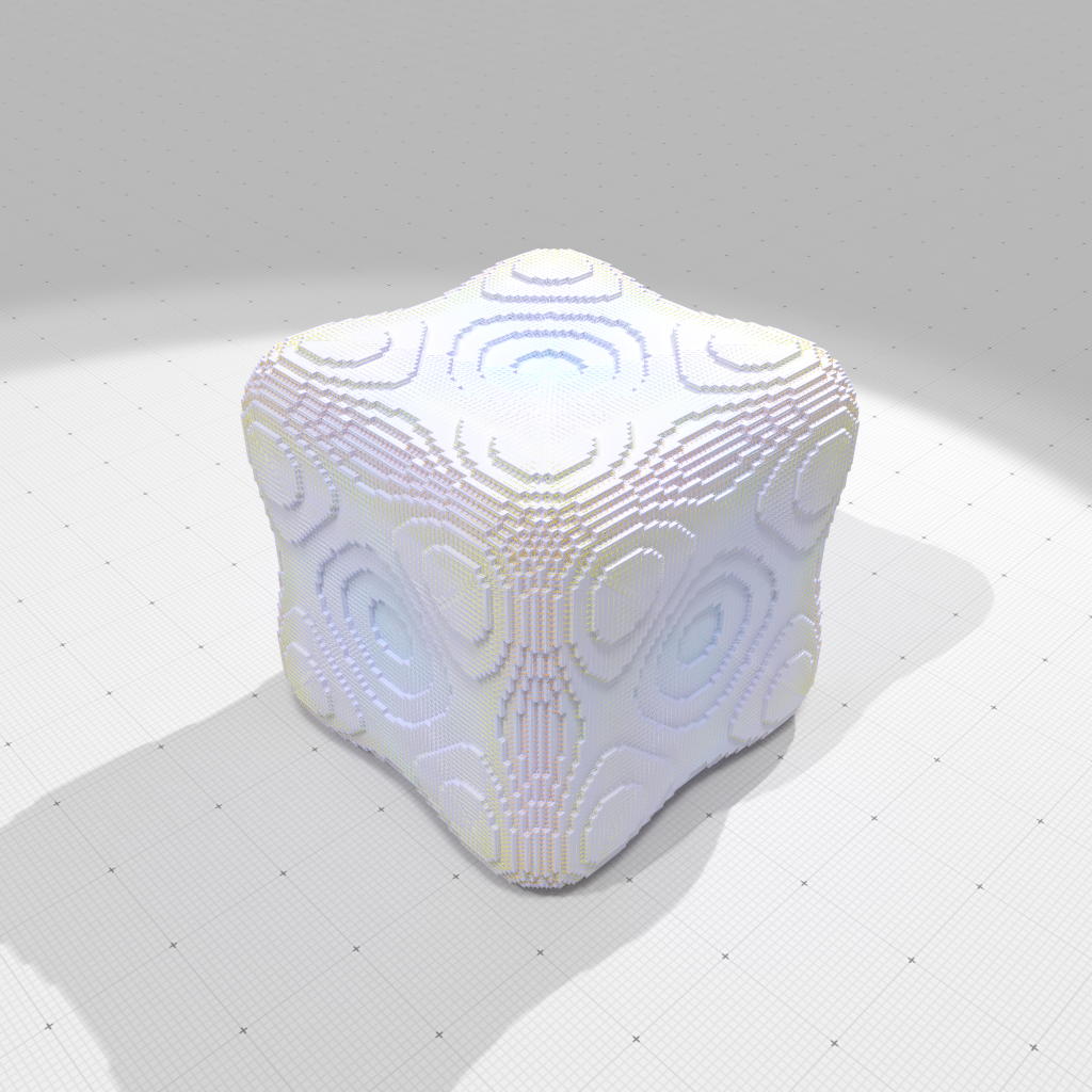
Principal directions of curvatures colored according to their value (blue negative, red positive) on goursat shape. |
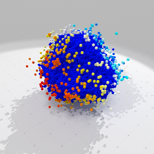
Load vol file -> Compute VoronoiMap -> Display distances to shape in viewer
This example requires ShortcutsGeometry and PolyscopeViewer. This shows how to compute distance to a shape using different metrics.
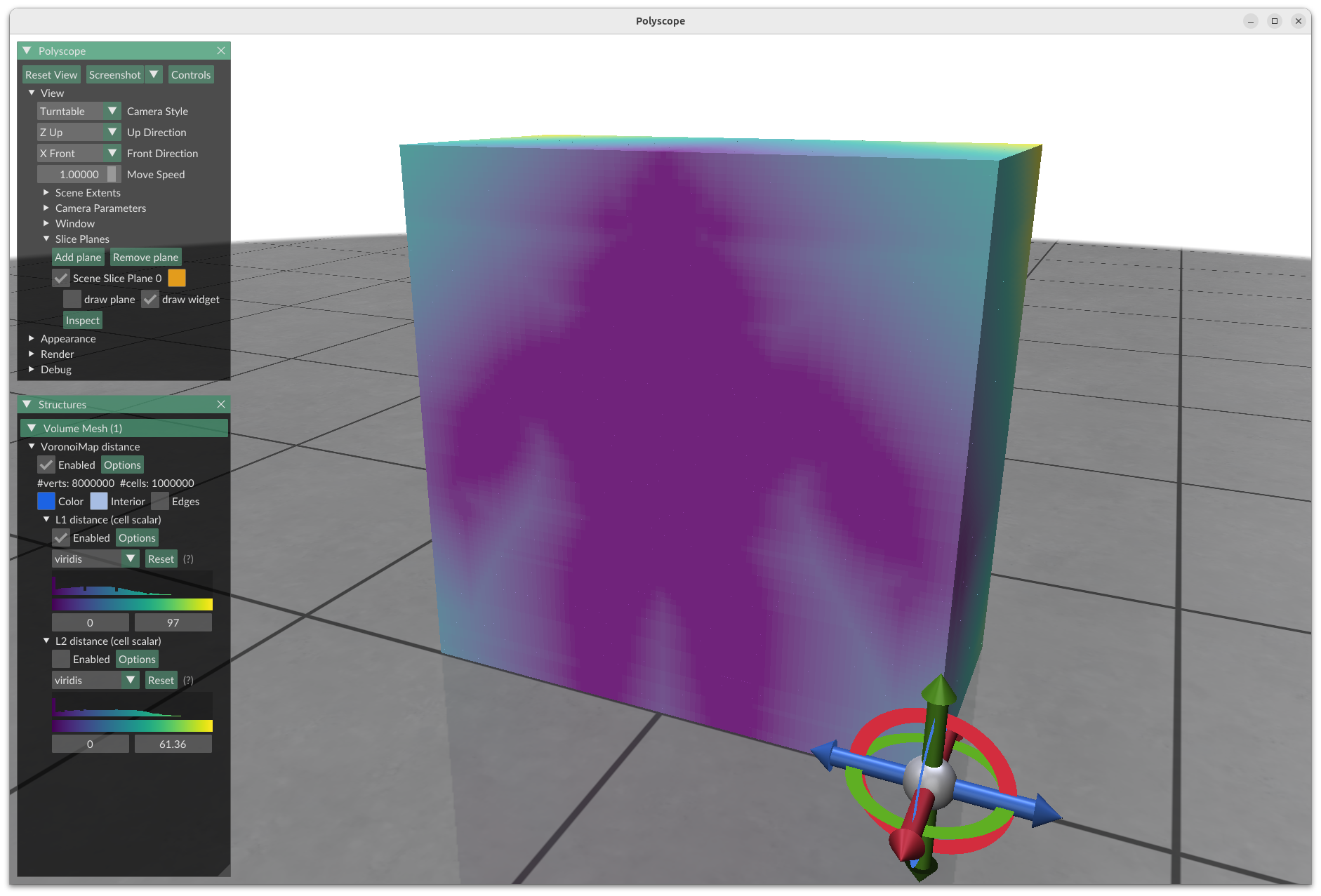
L1 distance to shape computed using VoronoiMap (image sliced within the viewer) | 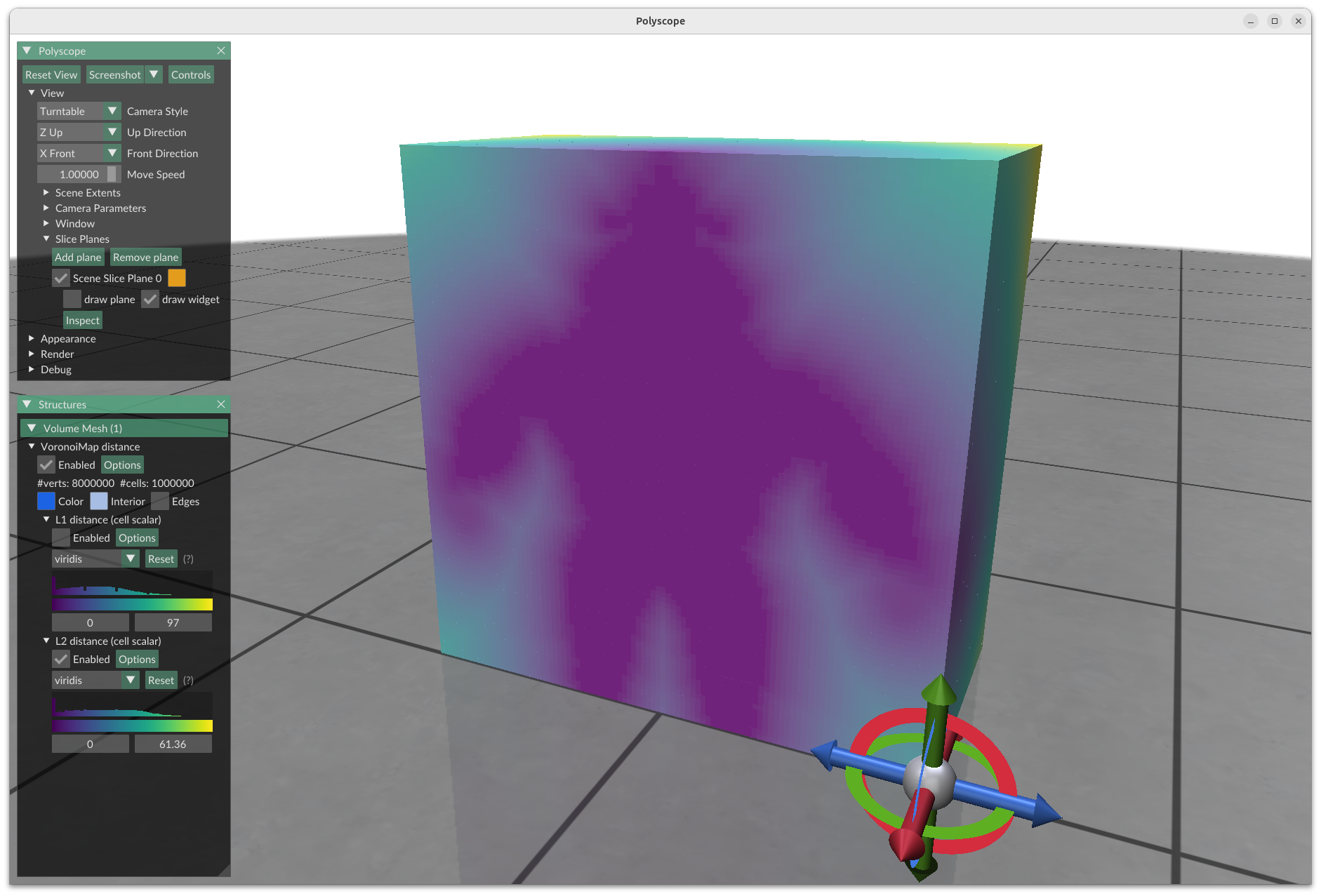
L2 distance to shape computed using VoronoiMap (image sliced within the viewer) |
Few 2D examples
We give below some minimalistic examples to show that shortcuts can save a lot of lines of code. All examples need at least the following lines:
Load pgm file -> ...
-> threshold -> save pgm
Philosophy and naming conventions
Commands are constructed as prefix + type name. Most of them are static methods and are overloaded to accept different set of parameters.
Prefixes
- make +
Type: means that it will create a new object of typeTypeand returns it as a smart pointer onto it. Depending on parameters, make can load a file, copy and transform an object, build an empty/not object according to parameters. - make +
Type+ s: means that it will create new objects of typeTypeand returns them as a vector of smart pointers onto it. - make +
Spec+Type: means that it will create a new object of typeTypewith some specialized meaning according toSpecand returns it as a smart pointer onto it. - save +
Type: means that it will save the pointed object of typeTypeas a file. - parameters +
Type: returns the Parameters object associated to the operations related to the givenType. - get +
Type: means that it will return by value an object of typeType.
Types
The following name conventions for types are used. They are defined according to your choice of cellular grid space when defining the Shortcuts type. For instance, if Z3i::KSpace was chosen, then Shortcuts::Point is Z3i::KSpace::Point.
- Shortcuts::Point: represents a point with integer coordinates.
- Shortcuts::Vector: represents a vector with integer coordinates.
- Shortcuts::RealPoint: represents a point with floating-point coordinates.
- Shortcuts::RealVector: represents a vector with floating-point coordinates.
- Shortcuts::Domain: represents an (hyper-)rectangular digital domain.
- Shortcuts::Integer: represents integer numbers (for Point coordinates and Vector components)
- Shortcuts::Space: represents a digital space (generally a SpaceND)
- Shortcuts::KSpace: represents a cellular grid space (generally a KhalimskySpaceND)
- Shortcuts::ImplicitShape3D: represents a functor RealPoint -> Scalar which adds geometry services: isInside, orientation, gradient, meanCurvature, GaussianCurvature, principalCurvatures, nearestPoint
- Shortcuts::DigitizedImplicitShape3D: represents the digitization of an ImplicitShape3D as a predicate Point -> bool (isInside), and adds some services: getLowerBound, getUpperBound, embed, round, getDomain, gridSteps, resolution. Note that pixels/voxels are not stored explicitly, so the resolution may be arbitrary high.
- Shortcuts::BinaryImage: represents a black and white image as an array of bits. It is generally a faster representation of a predicate Point -> bool than an implicit digital shape.
- Shortcuts::GrayScaleImage: represents an 8-bits gray-scale image as an array of bytes (unsigned char).
- Shortcuts::FloatImage: represents a float image as an array of floats.
- Shortcuts::DoubleImage: represents a double image as an array of doubles.
- Shortcuts::LightDigitalSurface: represents a connected digital surface over a binary image with an implicit representation.
- Shortcuts::DigitalSurface: represents an arbitrary digital surface with an explicit surfel set representation.
- Shortcuts::IdxDigitalSurface: represents an indexed digital surface with an explicit array-like representation.
- Shortcuts::Mesh: represents a simple mesh with arbitrary faces, but without topology (should be used when no surface topology is needed or when working with non-manifold surfaces).
- Shortcuts::TriangulatedSurface: represents a triangulated surface which may have boundaries (use HalfEdgeDataStructure).
- Shortcuts::PolygonalSurface: represents a polygonal surface which may have boundaries (use HalfEdgeDataStructure).
- Shortcuts::ColorMap: represents a colormap, i.e. a function assigning a color to a real value.
Main methods
- General methods
- Shortcuts::defaultParameters: returns the set of all shortcut parameters.
- Shortcuts::ImplicitShape3D methods
- Shortcuts::getPolynomialList: returns the list of polynomial shapes predefined for implicit shapes
- Shortcuts::parametersImplicitShape3D: parameters related to 3D implicit shapes (polynomial)
- Shortcuts::makeImplicitShape3D: builds a 3D implicit shape
- Shortcuts::KSpace methods
- Shortcuts::parametersKSpace: parameters related to Khalimsky spaces (closed)
- Shortcuts::getKSpace: overloaded methods for building a Khalimsky space from a domain or an image, from a bounding box, from a digitization process, or from a (indexed or not) digital surface.
- Shortcuts::refKSpace: overloaded methods for referencing the Khalimsky space of a (indexed or not) digital surface.
- Shortcuts::getCellEmbedder: returns the canonic cell embedder of the given space.
- Shortcuts::getSCellEmbedder: returns the canonic signed cell embedder of the given space.
- Shortcuts::DigitizedImplicitShape3D methods
- Shortcuts::parametersDigitizedImplicitShape3D: parameters related to shape digitization (bounding box, sampling)
- Shortcuts::makeDigitizedImplicitShape3D: digitizes an implicit shape.
- Shortcuts::BinaryImage methods
- Shortcuts::parametersBinaryImage: parameters related to binary images (noise, threshold).
- Shortcuts::makeBinaryImage: many overloaded methods for creating from scratch, vectorizing shape digitization, loading, copying/noisifying binary images, thresholding gray-scale images.
- Shortcuts::saveBinaryImage: saves a binary image to a file.
- Shortcuts::GrayScaleImage methods
- Shortcuts::makeGrayScaleImage: overloaded methods for creating from scratch or from binary image, or for loading gray scale images, or for creating a gray-scale image from a float or double image.
- Shortcuts::saveGrayScaleImage: saves a gray scale image to a file.
- Shortcuts::FloatImage methods
- Shortcuts::makeFloatImage: overloaded methods for creating a float image from a domain or from an implicit shape.
- Shortcuts::DoubleImage methods
- Shortcuts::makeDoubleImage: overloaded methods for creating a double image from a domain or from an implicit shape.
- Shortcuts::DigitalSurface methods
- Shortcuts::parametersDigitalSurface: parameters related to digital surfaces (surfel adjacency, components, internal heuristics)
- Shortcuts::getCellEmbedder: returns the canonic cell embedder of the given (indexed or not) digital surface
- Shortcuts::getSCellEmbedder: returns the canonic signed cell embedder of the given (indexed or not) digital surface.
- Shortcuts::makeLightDigitalSurface: creates a light connected surface around a (random) big enough component of a binary image
- Shortcuts::makeLightDigitalSurfaces: creates the vector of all light digital surfaces of the binary image or any one of its big components, can also output representant surfels
- Shortcuts::makeDigitalSurface: creates an arbitrary (connected or not) digital surface from a binary image, from a digitized implicit shape or from an indexed digital surface.
- Shortcuts::makeIdxDigitalSurface: creates an indexed digital surfaces that represents all the boundaries of a binary image or any one of its big components, or any given collection of surfels, or from light digital surface(s).
- Shortcuts::getSurfelRange: returns the surfels of a digital surface in the specified traversal order.
- Shortcuts::getCellRange: returns the k-dimensional cells of a digital surface in a the default traversal order (be careful, when it is not surfels, the order corresponds to the surfel order, and then to the incident cells).
- Shortcuts::getIdxSurfelRange: returns the indexed surfels of an indexed digital surface in the specified traversal order.
- Shortcuts::getPointelRange: returns the pointels of a digital surface in the default order and optionally the map Pointel -> Index giving the indices of each pointel, or simply the pointels around a surfel.
- Shortcuts::saveOBJ: several overloaded functions that save geometric elements as an OBJ file. You may save a digital surface as an OBJ file, with optionally positions, normals and colors information
- Shortcuts::RealVectors methods
- Shortcuts::saveVectorFieldOBJ: saves a vector field as an OBJ file (vectors are represented by tubes).
- Shortcuts::Mesh services
- Shortcuts::parametersMesh: parameters related to mesh, triangulated or polygonal surfaces.
- Shortcuts::makeTriangulatedSurface: builds the dual triangulated surface approximating an arbitrary digital surface, or the triangulated surface covering a given mesh, or subdivide a polygonal surface into a triangulated surface, or builds the marching cubes triangulated surface approximating an isosurface in a gray-scale image.
- Shortcuts::makePolygonalSurface: builds a polygonal surface from a mesh, or builds the marching cubes polygonal surface approximating an isosurface in a gray-scale image.
- Shortcuts::makePrimalPolygonalSurface: builds the primal polygonal surface of a (manifold) digital surface
- Shortcuts::makePrimalSurfaceMesh: builds the primal polygonal surface of a digital surface (which may contain non-manifold edges)
- Shortcuts::makeDualPolygonalSurface: builds the dual polygonal surface of a digital surface
- Shortcuts::makeSurfaceMesh: load a surface mesh from file
- Shortcuts::saveOBJ: saves a triangulated or polygonal surface or a mesh as an OBJ file, with optionally normals and colors information.
- ShortcutsGeometry::Mesh utilities
- Shortcuts::parametersUtilities: parameters related to colormaps.
- Shortcuts::getColorMap: returns the specified colormap.
- Shortcuts::getZeroTickedColorMap: returns the specified colormap with a tic around zero.
- Shortcuts::getRangeMatch: returns the perfect or approximate match/correspondence between two ranges.
- Shortcuts::getMatchedRange: returns the perfectly or approximately matched/corresponding range.
- Shortcuts::getPrimalVertices: returns the vertices (possibly consistently ordered along the face) of the given signed cell.
- Shortcuts::outputSurfelsAsObj: outputs surfels in standard OBJ file format.
- Shortcuts::outputPrimalDigitalSurfaceAsObj: outputs any digital surface in standard OBJ file format as its primal quadrangulated mesh.
- Shortcuts::outputPrimalIdxDigitalSurfaceAsObj: outputs any indexed digital surface in standard OBJ file format as its primal quadrangulated mesh.
- Shortcuts::outputDualDigitalSurfaceAsObj: outputs any digital surface in standard OBJ file format as its dual polygonal or triangulated mesh.
- Shape Geometry services
- ShortcutsGeometry::parametersShapeGeometry: parameters related to implicit shape geometry.
- ShortcutsGeometry::getPositions: returns the positions on the 3D implicit shape close to the specified surfels.
- ShortcutsGeometry::getNormalVectors: returns the vectors normal to the 3D implicit shape close to the specified surfels.
- ShortcutsGeometry::getMeanCurvatures: returns the mean curvatures along the 3D implicit shape close to the specified surfels.
- ShortcutsGeometry::getGaussianCurvatures: returns the Gaussian curvatures along the 3D implicit shape close to the specified surfels.
- ShortcutsGeometry::getFirstPrincipalCurvatures: returns the first (smallest) principal curvatures along the 3D implicit shape close to the specified surfels.
- ShortcutsGeometry::getSecondPrincipalCurvatures: returns the second (greatest) principal curvatures along the 3D implicit shape close to the specified surfels.
- ShortcutsGeometry::getFirstPrincipalDirections: returns the first principal directions along the 3D implicit shape close to the specified surfels.
- ShortcutsGeometry::getSecondPrincipalDirections: returns the second principal directions along the 3D implicit shape close to the specified surfels.
- ShortcutsGeometry::getPrincipalCurvaturesAndDirections: returns the first and second principal curvatures and directions along the 3D implicit shape close to the specified surfels.
- Geometry Estimation services
- ShortcutsGeometry::parametersGeometryEstimation: parameters related to geometric estimators.
- ShortcutsGeometry::getTrivialNormalVectors: returns the trivial (Trivial) normal vectors to the given surfel range
- ShortcutsGeometry::getCTrivialNormalVectors: returns the convolved trivial (CTrivial) normal vectors to the given surfel range
- ShortcutsGeometry::getVCMNormalVectors: returns the Voronoi Covariance Measure (VCM) normal vectors to the given surfel range
- ShortcutsGeometry::getIINormalVectors: returns the Integral Invariant (II) normal vectors to the given surfel range (embedded in a binary image or a digitized implicit shape)
- ShortcutsGeometry::getIIMeanCurvatures: returns the Integral Invariant (II) mean curvatures onto the given surfel range (embedded in a binary image or a digitized implicit shape)
- ShortcutsGeometry::getIIGaussianCurvatures: returns the Integral Invariant (II) Gaussian curvatures onto the given surfel range (embedded in a binary image or a digitized implicit shape)
- ShortcutsGeometry::getIIPrincipalCurvaturesAndDirections: returns the Integral Invariant (II) principal curvatures values and directions for the given surfel range (embedded in a binary image or a digitized implicit shape)
- ShortcutsGeometry::getCNCMeanCurvatures: returns the Corrected Normal Current (CNC) mean curvatures onto the given faces (as ids of the mesh).
- ShortcutsGeometry::getCNCGaussianCurvatures: returns the Corrected Normal Current (CNC) gaussian curvatures onto the given faces (as ids of the mesh).
- ShortcutsGeometry::getCNCPrincipalCurvaturesAndDirections: returns the Corrected Normal Current (CNC) principal curvatures values and directions for the given face range (as ids of the mesh).
- ShortcutsGeometry::orientVectors: reorient a range of vectors so as to point in the same half-space as another range of vectors.
- Volumetric services
- ShortcutsGeometry::getVoronoiMap: return the Voronoi map on a domain from a list of sites
- ShortcutsGeometry::getDistanceTransformation: return the distance transformation on a domain from a list of sites
- ShortcutsGeometry::getDirectionToClosestSite: return the list of vectors to the closest site
- ShortcutsGeometry::getDistanceToClosestSite: return the distance to the closest site
- ShortcutsGeometry::getRAwDistanceToClosestSite: return the (raw) distance to the closest site. Raw distance means an exact representation of the distance value from integers dropping the 1/p exponent for Lp metrics (i.e. squared distance for the Euclidean L2 metric)
- AT Approximation services
- ShortcutsGeometry::parametersATApproximation: parameters related to piecewise-smooth AT approximation.
- ShortcutsGeometry::getATVectorFieldApproximation: returns the piecewise-smooth approximation of the given vector field, and optionally returns the locii of discontinuity
- Misc. services
- ShortcutsGeometry::getScalarsAbsoluteDifference: return the range of scalars that is the difference of two range of scalars
- ShortcutsGeometry::getVectorsAngleDeviation: return the range of scalars that form the angle deviations between two range of vectors
- ShortcutsGeometry::getStatistic: return the statistic of the given range of values.
Parameters
In all methods, out parameters are listed before in parameters. Also, methods whose result can be influenced by global parameters are parameterized through a Parameters object. Hence static methods follow this pattern:
<return-type> Shortcuts::fonction-name ( [ <out-parameter(s)> ], [ <in-parameter(s)> ], [ Parameters params ] )
The simplest way to get default values for global parameters is to start with a line:
And then to change your parameter settings with Parameters::operator(), for instance:
You also have the bitwise-or (operator|) to merge Parameters.