Table of Contents
- Author(s) of this documentation:
- Jacques-Olivier Lachaud
- Since
- 1.3
Part of the Geometry package.
This part of the manual describes the implementation of several curvature measures on quite arbitrary meshes (any instance of SurfaceMesh). The classical curvature measures related to the Normal Cycle are provided as well as the more general curvature measures based on corrected normal currents. This module implements the research on corrected normal currents presented in papers [76] and [77], and also gives a stand-alone implementation of the normal cycle method, which was presented in papers [37] and [38].
The following programs are related to this documentation: geometry/meshes/curvature-measures-icnc-3d.cpp, geometry/meshes/curvature-measures-icnc-XY-3d.cpp, geometry/meshes/curvature-measures-nc-3d.cpp, geometry/meshes/curvature-measures-nc-XY-3d.cpp, geometry/meshes/obj-curvature-measures-icnc-3d.cpp, geometry/meshes/obj-curvature-measures-icnc-XY-3d.cpp, geometry/meshes/vol-curvature-measures-icnc-3d.cpp, geometry/meshes/vol-curvature-measures-icnc-XY-3d.cpp, geometry/meshes/digpoly-curvature-measures-cnc-3d.cpp, geometry/meshes/digpoly-curvature-measures-cnc-XY-3d.cpp.
The following tests are related to this documentation: testCorrectedNormalCurrentComputer.cpp, testNormalCycleComputer.cpp.
Introduction to curvature measures
Curvature is an important geometric piece of information which has the drawback of being well defined only on smooth sets. Unfortunately, most geometric data are non-smooth (e.g. triangulated or polygonal surfaces, point clouds, polyhedra). A lot of works have thus aimed at generalizing curvatures to such sets, while guaranteeing that such definitions tend (in some sense) towards the classical smooth curvatures when working on finer and finer non smooth approximations of smooth data.
The seminal paper of Federer [52] first defined curvature measures on sets with positive reach (which includes smooth and convex polyhedra, but not triangulated surfaces in general). Using the notion of Normal Cycle introduced by Wintgen [122], the curvature measure principle was then extended to a wider class of objects including triangulations, digitized objects and subanalytic sets by Fu [60].
The main idea of the Normal Cycle is to embed the shape into the Grassmann bundle, which encodes both positions and the normal cones. This embedding is itself piecewise smooth, and curvatures can be defined onto it by integration with the invariant differential forms (Lipschitz-Killing forms). This approach was used for instance by Cohen-Steiner and Morvan [37] [38] for triangulated surfaces, where they show stability of curvature measures for surface sampling with convergent normals. Extensions of such works to point clouds using offset surfaces were proposed by Chazal, Cohen-Steiner, Lieutier and Thibert in [25].
However these methods do not provide consistent curvature estimates when the normal vector field of the discretization does not tend towards the normal vector field of the reference smooth surface. A famous example is the Schwarz lantern. This is also the case of digital surfaces that are boundaries of pixel/voxel data in images. For these surfaces, even high resolution data implies only 4 (in 2D) or 6 (in 3D) possible normal vectors.
This module therefore proposes an implementation of corrected normal currents to compute curvature measures onto quite general discrete surface data. The key idea is to replace the normal vector field of a surface S by another vector field u which we assume to be geometrically more meaningful. For instance if S is a digitization of a smooth surface X, one may take for u a local average of the naive normals of X.
The general theory was proposed by Lachaud, Romon and Thibert in [76]. It deals with piecewise \( C^{1,1} \) surfaces, with piecewise \( C^1 \) corrected normal vector field. A specialized version restricted to polygonal meshes equipped with a normal vector field defined by linear interpolation was presented in [77], and leads to quite simple formulae.
For instance, the interpolated corrected curvature measures take the following values on a triangle \( \tau_{ijk} \), with vertices i, j, k:
\[ \begin{align*} \mu^{(0)}(\tau_{ijk}) = &\frac{1}{2} \langle \bar{\mathbf{u}} \mid (\mathbf{x}_j - \mathbf{x}_i) \times (\mathbf{x}_k - \mathbf{x}_i) \rangle, \\ \mu^{(1)}(\tau_{ijk}) = &\frac{1}{2} \langle \bar{\mathbf{u}} \mid (\mathbf{u}_k - \mathbf{u}_j) \times \mathbf{x}_i + (\mathbf{u}_i - \mathbf{u}_k) \times \mathbf{x}_j + (\mathbf{u}_j - \mathbf{u}_i) \times \mathbf{x}_k \rangle, \\ \mu^{(2)}(\tau_{ijk}) = &\frac{1}{2} \langle \mathbf{u}_i \mid \mathbf{u}_j \times \mathbf{u}_k \rangle, \\ \mu^{\mathbf{X},\mathbf{Y}}(\tau_{ijk}) = & \frac{1}{2} \big\langle \bar{\mathbf{u}} \big| \langle \mathbf{Y} | \mathbf{u}_k -\mathbf{u}_i \rangle \mathbf{X} \times (\mathbf{x}_j - \mathbf{x}_i) \big\rangle -\frac{1}{2} \big\langle \bar{\mathbf{u}} \big| \langle \mathbf{Y} | \mathbf{u}_j -\mathbf{u}_i \rangle \mathbf{X} \times (\mathbf{x}_k - \mathbf{x}_i) \big\rangle, \end{align*} \]
where \( \langle \cdot \mid \cdot \rangle \) denotes the usual scalar product, \( \bar{\mathbf{u}}=\frac{1}{3}( \mathbf{u}_i + \mathbf{u}_j + \mathbf{u}_k )\).
The measure \( \mu^{(0)} \) is the corrected area density of the given triangle, \( \mu^{(1)} \) is twice its corrected mean curvature density, \( \mu^{(2)} \) is its corrected Gaussian curvature density. The (anisotropic) measure \( \mu^{\mathbf{X},\mathbf{Y}} \) is the trace of the corrected second fundamental form along directions \( \mathbf{X} \) and \( \mathbf{Y} \). While the smooth second fundamental form is naturally a symmetric 2-tensor, there is no easy way to define tangent directions at a vertex, so the anisotropic measure depends on two 3D vectors; when \( \mathbf{X} \) and \( \mathbf{Y} \) are tangent, \( \mu^{\mathbf{X},\mathbf{Y}} \) is close to the second fundamental form applied to these vectors, while its value along normal direction tends to zero asymptotically.
These measures are naturally extended to an arbitrary subset B of \( \mathbb{R}^3 \) by measuring its intersection ratio with each triangle \( \tau \) and by suming over all triangles of the mesh.
\[ \mu^{(k)}( B ) = \sum_{\tau : \text{triangle} } \mu^{(k)}( \tau ) \frac{\mathrm{Area}( \tau \cap B )}{\mathrm{Area}(\tau)}. \]
Computing curvature measures on meshes
Curvature measures formula per triangle/edge/vertex are provided in class NormalCycleFormula (for the curvatures measures induced by the Normal Cycle) and in class CorrectedNormalCurrentFormula (for the curvatures measures induced by corrected normal currents with interpolated corrected normal vector field).
However one generally wishes to compute the measures over a mesh in a ball of given center and radius. It is then more convenient to use classes NormalCycleComputer and CorrectedNormalCurrentComputer, which are dedicated to compute curvature measures over a SurfaceMesh object.
Normal Cycle curvature measures
You may proceed as follows (see examples geometry/meshes/curvature-measures-nc-3d.cpp and geometry/meshes/curvature-measures-nc-XY-3d.cpp).
You need to include header file of class NormalCycleComputer:
then use some typedefs adapted to your problem.
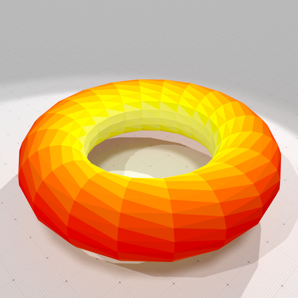
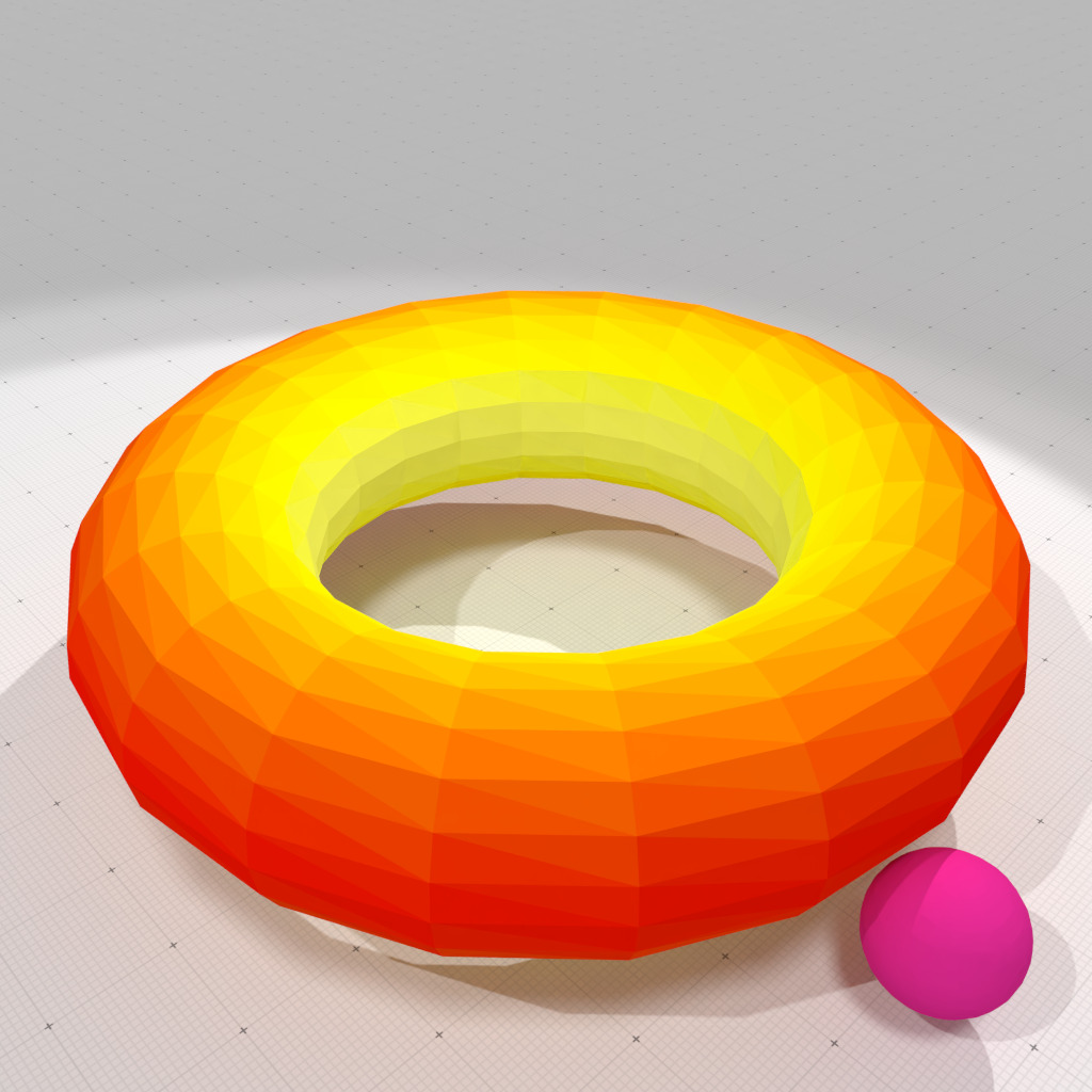
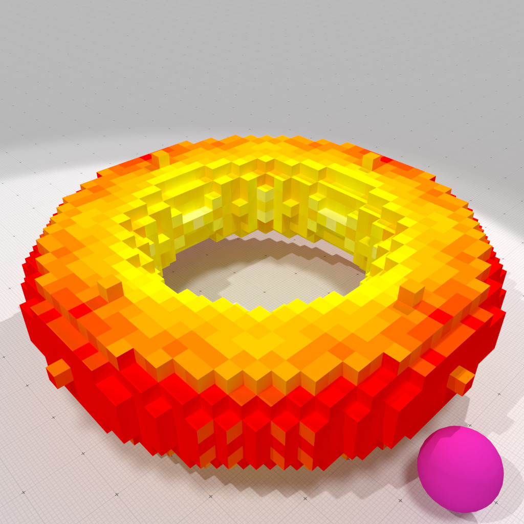
We will compute curvature measures onto a SurfaceMesh object. Here, we build a torus of big radius 3 and small radius 1, with a discretization of 20x20.
It is not necessary here to equip the mesh with normals, since the Normal Cycle infers the normals from the positions of the mesh. We can now compute three measures onto the mesh, mu0 the area measure, mu1 twice the mean curvature measure, and mu2 the Gaussian curvature measure. You have static methods NormalCycleComputer::meanCurvature and NormalCycleComputer::GaussianCurvature that estimate respectively mean and Gaussian curvature from measures.
Normal cycle mean and Gaussian curvature measures have meaning only around edges and vertices. So it is necessary to measure them in a big enough ball that includes at least one edge or vertex, and then to normalize the result by dividing by the area measure. Therefore, if we wish to estimate mean and Gaussian curvatures at every face centroid (say), the following snippet shows how to do it, assuming a measuring ball radius of R:
This is is the result for a measuring ball radius of 0.5 onto the torus shape.
Expected mean curvatures: min=0.25 max=0.625
Computed mean curvatures: min=0.189446 max=0.772277
Expected Gaussian curvatures: min=-0.5 max=0.25
Computed Gaussian curvatures: min=-0.682996 max=0.547296
A quite similar code allows you to compute anisotropic curvature measures (i.e. a kind of second fundamental form). You may extract from the returned tensor measure (using eigenvalues/eigenvectors) principal curvatures and principal directions, by using method NormalCycleComputer::principalCurvatures.
Expected k1 curvatures: min=-0.5 max=0.25
Computed k1 curvatures: min=-0.581281 max=0.441977
Expected k2 curvatures: min=1 max=1
Computed k2 curvatures: min=0.904081 max=1.06404
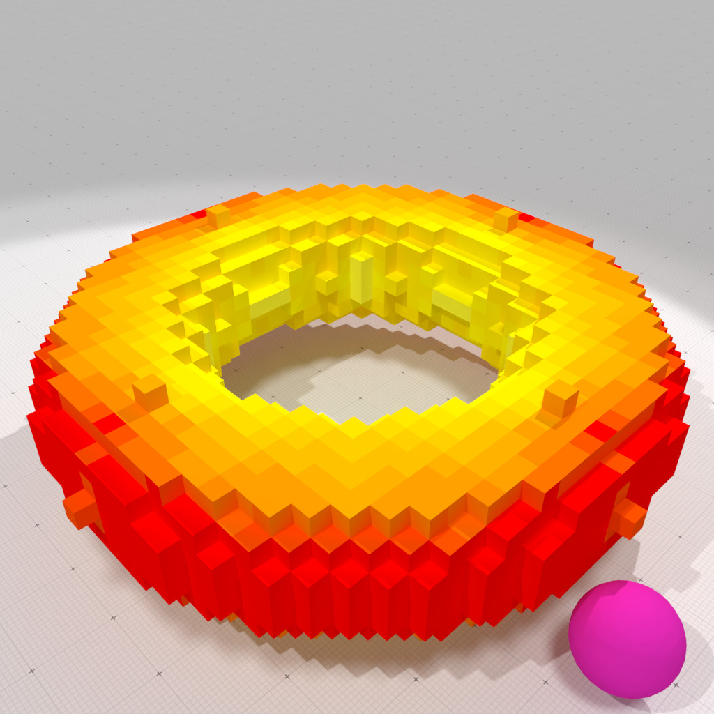
Curvature estimates are displayed with a colormap [-0.625 ... 0 ... 0.625] -> [Blue ... White ... Red].
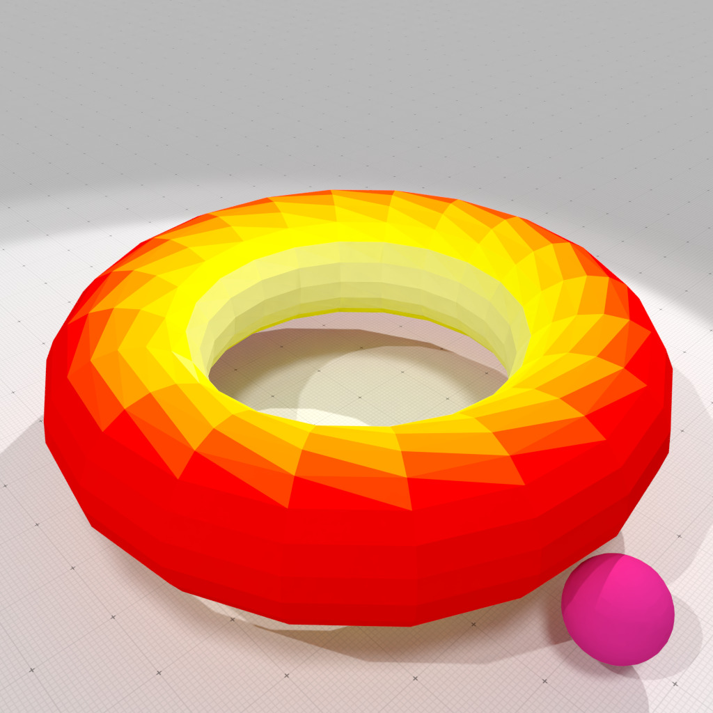
Normal cycle mean curvature measure, r=0.5 | 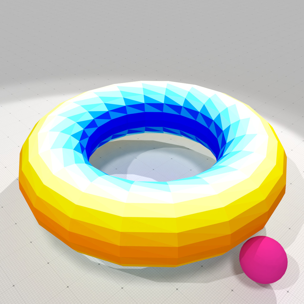
Normal cycle Gaussian curvature measure, r=0.5 | 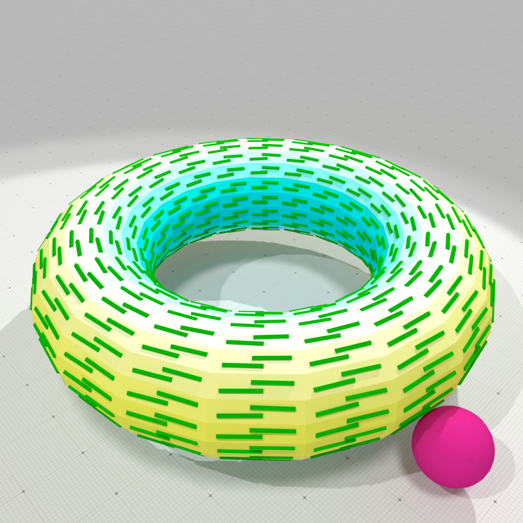
Normal cycle smallest principal curvature and direction, r=0.5 | 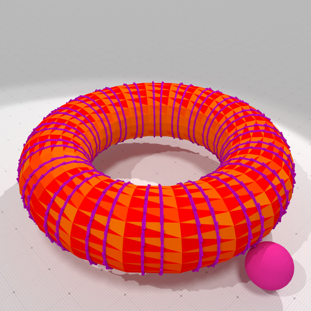
Normal cycle greatest principal curvature and direction, r=0.5 |
Interpolated Corrected Normal Current curvature measures
You may proceed as follows (see examples geometry/meshes/curvature-measures-icnc-3d.cpp and geometry/meshes/curvature-measures-icnc-XY-3d.cpp).
You need to include header file of class CorrectedNormalCurrentComputer:
then use some typedefs adapted to your problem.
We will compute curvature measures onto a SurfaceMesh object. Here, we build a torus of big radius 3 and small radius 1, with a discretization of 20x20.
- Warning
- It is necessary here to equip the mesh with normals, since the Corrected NormalCurrent needs a corrected vector field to compute curvatures.
Here we just provide the corrected normal vector field \( \mathbf{u}
\) as a normal vector per vertex, the field is then linearly interpolated. We can now compute three measures onto the mesh, mu0 the area measure, mu1 twice the mean curvature measure, and mu2 the Gaussian curvature measure. You have static methods CorrectedNormalCurrentComputer::meanCurvature and CorrectedNormalCurrentComputer::GaussianCurvature that estimate respectively mean and Gaussian curvature from measures.
A big advantage of (interpolated) Corrected Normal Current over Normal Cycle is that the induced mean and Gaussian curvature measures have meaning for arbitrary measuring set (even when the area of the set tends to zero. Therefore, if we wish to estimate mean and Gaussian curvatures at every face centroid (say), the following snippet shows how to do it, assuming a measuring ball radius of R:
This is is the result for a measuring ball radius of 0.0 onto the torus shape (perfect results !).
Expected mean curvatures: min=0.25 max=0.625
Computed mean curvatures: min=0.25 max=0.625
Expected Gaussian curvatures: min=-0.5 max=0.25
Computed Gaussian curvatures: min=-0.5 max=0.25
This is is the result for a measuring ball radius of 0.5 onto the torus shape (better than Normal cycle).
Expected mean curvatures: min=0.25 max=0.625
Computed mean curvatures: min=0.264763 max=0.622318
Expected Gaussian curvatures: min=-0.5 max=0.25
Computed Gaussian curvatures: min=-0.470473 max=0.244636
A quite similar code allows you to compute anisotropic curvature measures (i.e. a kind of second fundamental form). You may extract from the returned tensor measure (using eigenvalues/eigenvectors) principal curvatures and principal directions, by using method CorrectedNormalCurrentComputer::principalCurvatures.
This gives you such results for principal curvatures estimations, first for a radius 0:
Expected k1 curvatures: min=-0.5 max=0.25
Computed k1 curvatures: min=-0.500225 max=0.249888
Expected k2 curvatures: min=1 max=1
Computed k2 curvatures: min=1.00011 max=1.00678
then for a radius of 0.5:
Expected k1 curvatures: min=-0.5 max=0.25
Computed k1 curvatures: min=-0.454026 max=0.242436
Expected k2 curvatures: min=1 max=1
Computed k2 curvatures: min=0.924283 max=0.95338
Curvature estimates are displayed with a colormap [-0.625 ... 0 ... 0.625] -> [Blue ... White ... Red].
Corrected Normal Current mean curvature measure, r=0 | 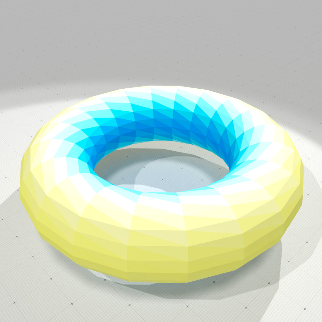
Corrected Normal Current Gaussian curvature measure, r=0 | 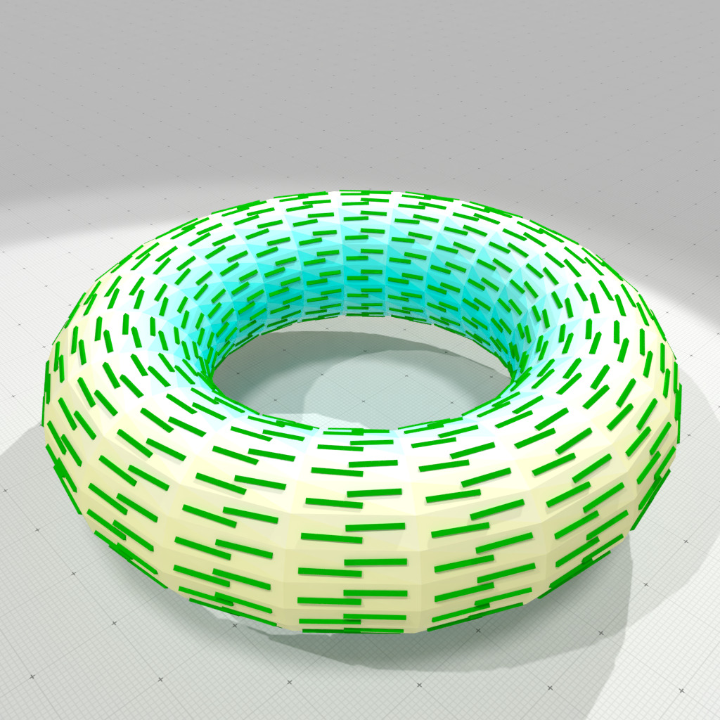
Corrected Normal Current smallest principal curvature and direction, r=0 | 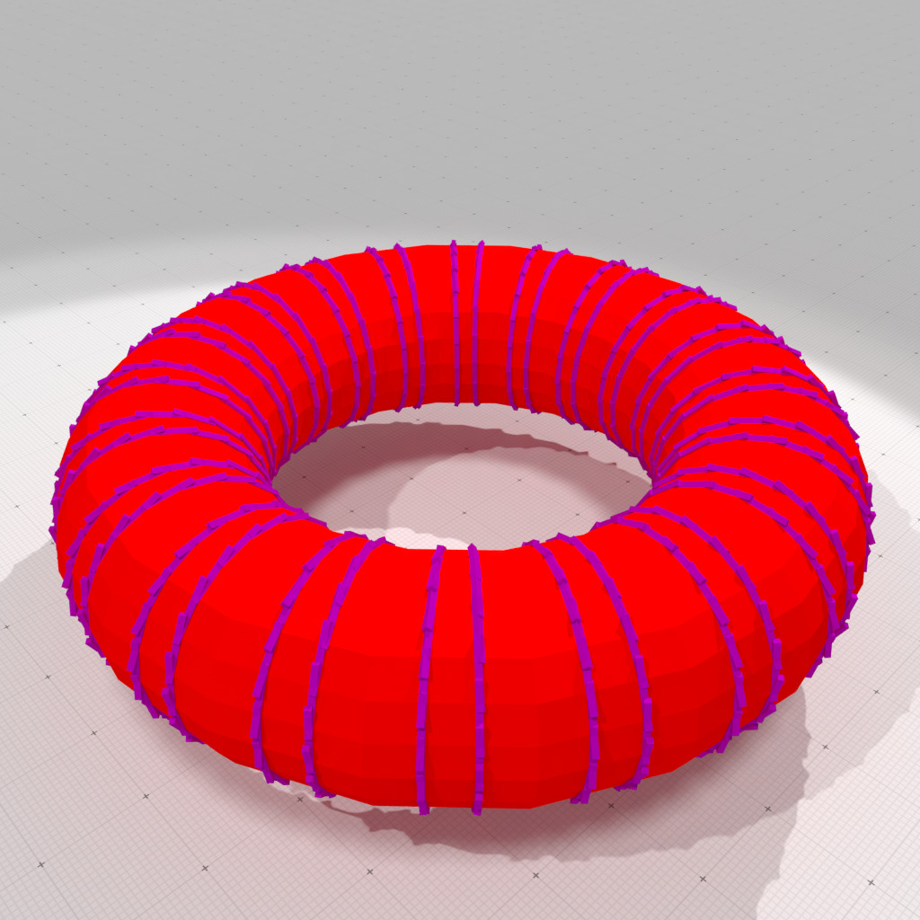
Corrected Normal Current greatest principal curvature and direction, r=0 |
Corrected Normal Current mean curvature measure, r=0.5 | 
Corrected Normal Current Gaussian curvature measure, r=0.5 | 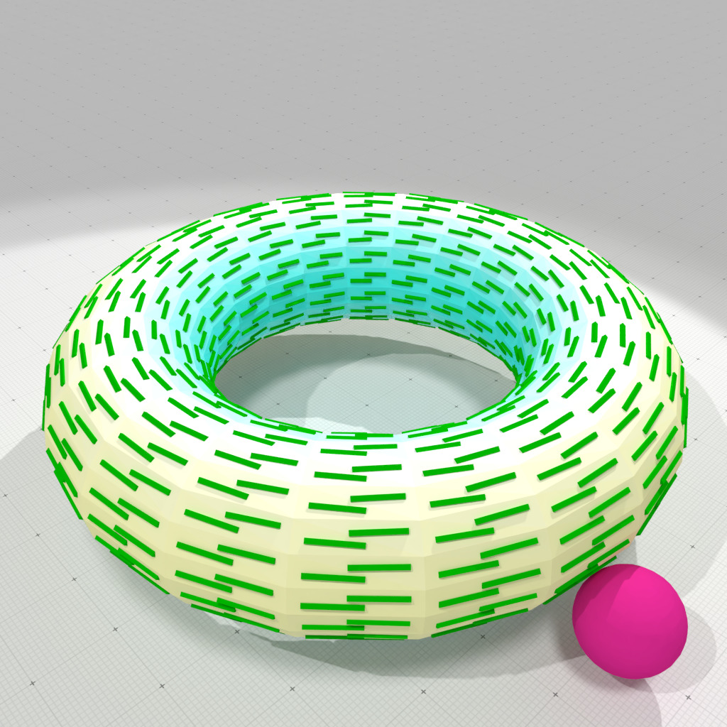
Corrected Normal Current smallest principal curvature and direction, r=0.5 | 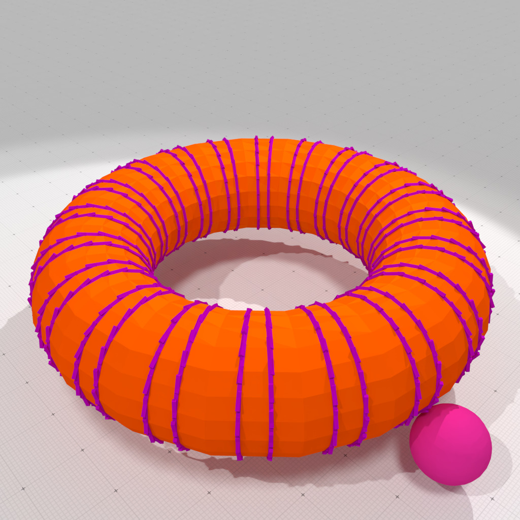
Corrected Normal Current greatest principal curvature and direction, r=0.5 |
- Note
- You may check that Normal Cycle fails on the Schwarz lantern, while interpolated Corrected Normal Current provides the correct curvature estimation.
./examples/geometry/meshes/curvature-measures-nc-3d lantern 20 20 0.5outputs Expected mean curvatures: min=0.25 max=0.25 Computed mean curvatures: min=0.795695 max=1.41211 Expected Gaussian curvatures: min=0 max=0 Computed Gaussian curvatures: min=-6.79045e-14 max=15.0937 | ./examples/geometry/meshes/curvature-measures-icnc-3d lantern 20 20 0.5outputs Expected mean curvatures: min=0.25 max=0.25 Computed mean curvatures: min=0.25 max=0.25 Expected Gaussian curvatures: min=0 max=0 Computed Gaussian curvatures: min=0 max=0 |
Vertex-interpolated versus face-constant corrected normal current
The theory of corrected normal currents works for arbitrary piecewise smooth corrected normal vector fields. Class CorrectedNormalCurrentComputer allows you to choose between a constant per face corrected normal vector field (called Constant Corrected Normal Current, CCNC), or a smooth corrected normal vector field obtained by linear interpolation of vertex normals per face (called Interpolated Corrected Normal Current, ICNC).
The choice is made automatically by the CorrectedNormalCurrentComputer object according to the user-defined normal vector field of its associated SurfaceMesh object:
- if
myMesh.vertexNormals()is not empty, then the CorrectedNormalCurrentComputer computes ICNC measures, - otherwise if
myMesh.faceNormals()is not empty, then the CorrectedNormalCurrentComputer computes CCNC measures, - otherwise the CNC does not work and outputs a warning.
For instance, you may force ICNC on a mesh as follows:
Otherwise, assume you have not set any vertex normals, the following code uses CCNC:
- Warning
- As Normal Cycle curvature measures, face-constant CNC (CCNC) curvature measures require a minimum radius for the measuring ball. Indeed, its \( \mu^{(1)} \) and \( \mu^{(\mathbf{X},\mathbf{Y})} \) measures must capture at least one edge, while its \( \mu^{(2)} \) measure must capture at least one vertex. In opposition to CCNC and NC, vertex-interpolated CNC curvature measures (ICNC) are valid for arbitrary radius. All the ICNC curvatures have a well-defined limit when the measuring set radius tends to zero.
More on curvature measures
NormalCycleComputer and CorrectedNormalCurrentComputer provides methods that return measures, more precisely as SurfaceMeshMeasure objects. The values of measure may be arbitrary scalars, vectors or tensors. Here curvature measures are either scalars (like area, mean and Gaussian curvature measures) or tensors (anisotropic measures).
A SurfaceMeshMeasure provides several handy methods to evaluate measures wrt simple subsets of \( \mathbb{R}^3 \).
- SurfaceMeshMeasure::measure() const returns the total measure, i.e. \( \mu(\mathbb{R^3}) \).
- SurfaceMeshMeasure::measure( const RealPoint&, Scalar, Face ) const computes the measure \( \mu(B_r(x)) \), where \( B_r(x) \) is the ball of center x and radius r. The center x must lie on or close to the face f.
- Note
- The measures may be associated to 0-, 1-, 2- cells, but generally you do not require this level of detail. If you prefer to have direct access to these measures, you have several overloaded methods to do this: SurfaceMeshMeasure::vertexMeasure, SurfaceMeshMeasure::edgeMeasure, SurfaceMeshMeasure::faceMeasure. They can accept weighted sum of cells as input.
ICNC Curvature computation on OBJ surface
Examples geometry/meshes/obj-curvature-measures-icnc-3d.cpp and geometry/meshes/obj-curvature-measures-icnc-XY-3d.cpp show how to compute all curvature information on an arbitrary mesh.
The only difference in the above examples is the way the SurfaceMesh object is created. Here we read an OBJ file to create it.
Remember that a SurfaceMesh object may represent a non-manifold polygonal surface.
Once the mesh is created, you just need to ensure that the SurfaceMesh object has a normal vector attached to each of its vertex. This can be done as follows (or just provide an OBJ file with vertex normals):
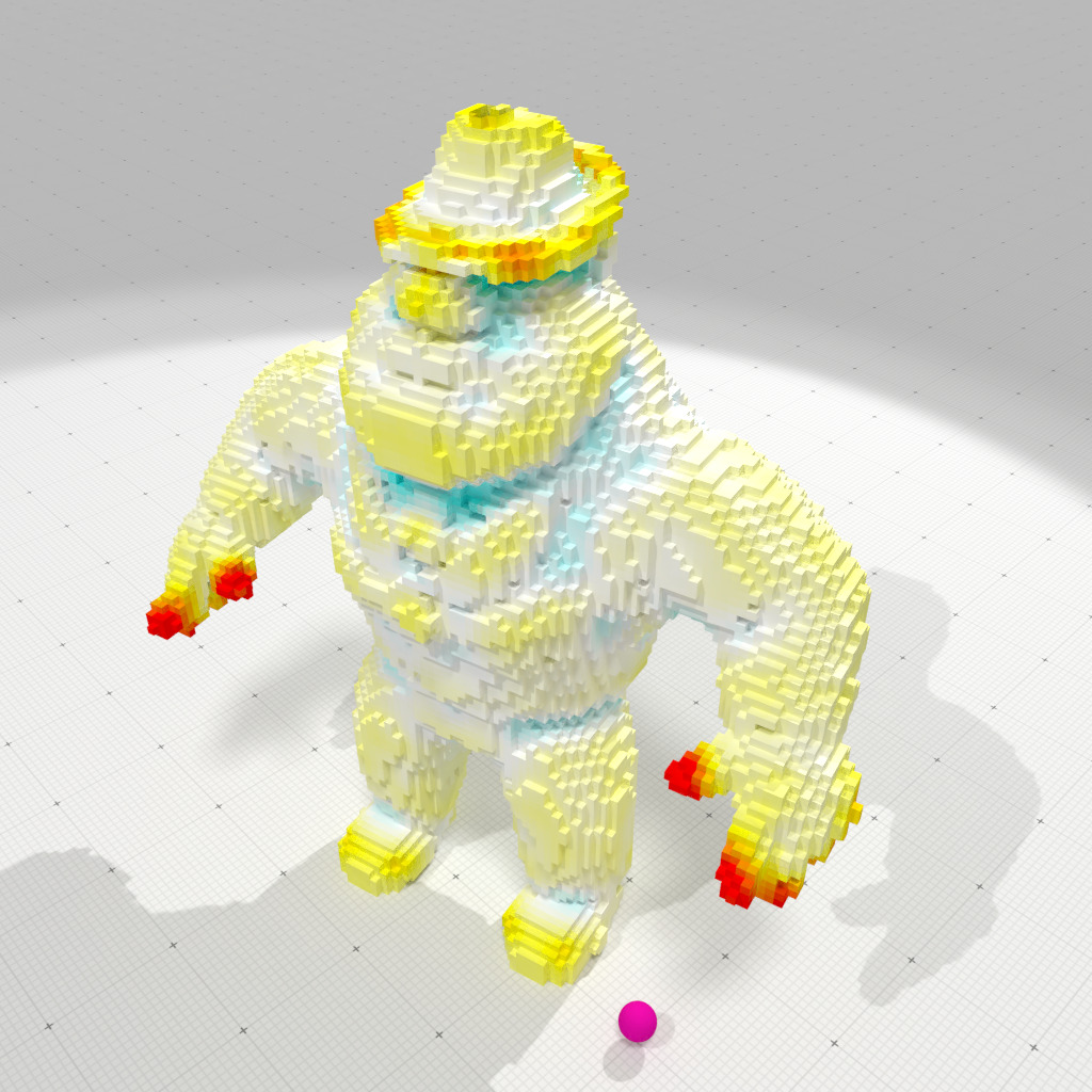
The rest of the code is identical. The two examples gives the following curvature estimates on "spot.obj" file.
Interpolated corrected mean curvature measure, r=0.05 | 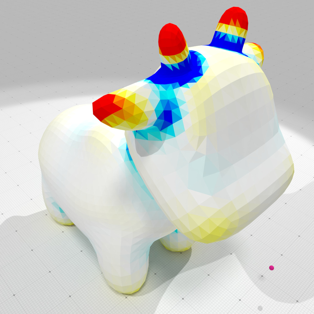
Interpolated corrected Gaussian curvature measure, r=0.05 | 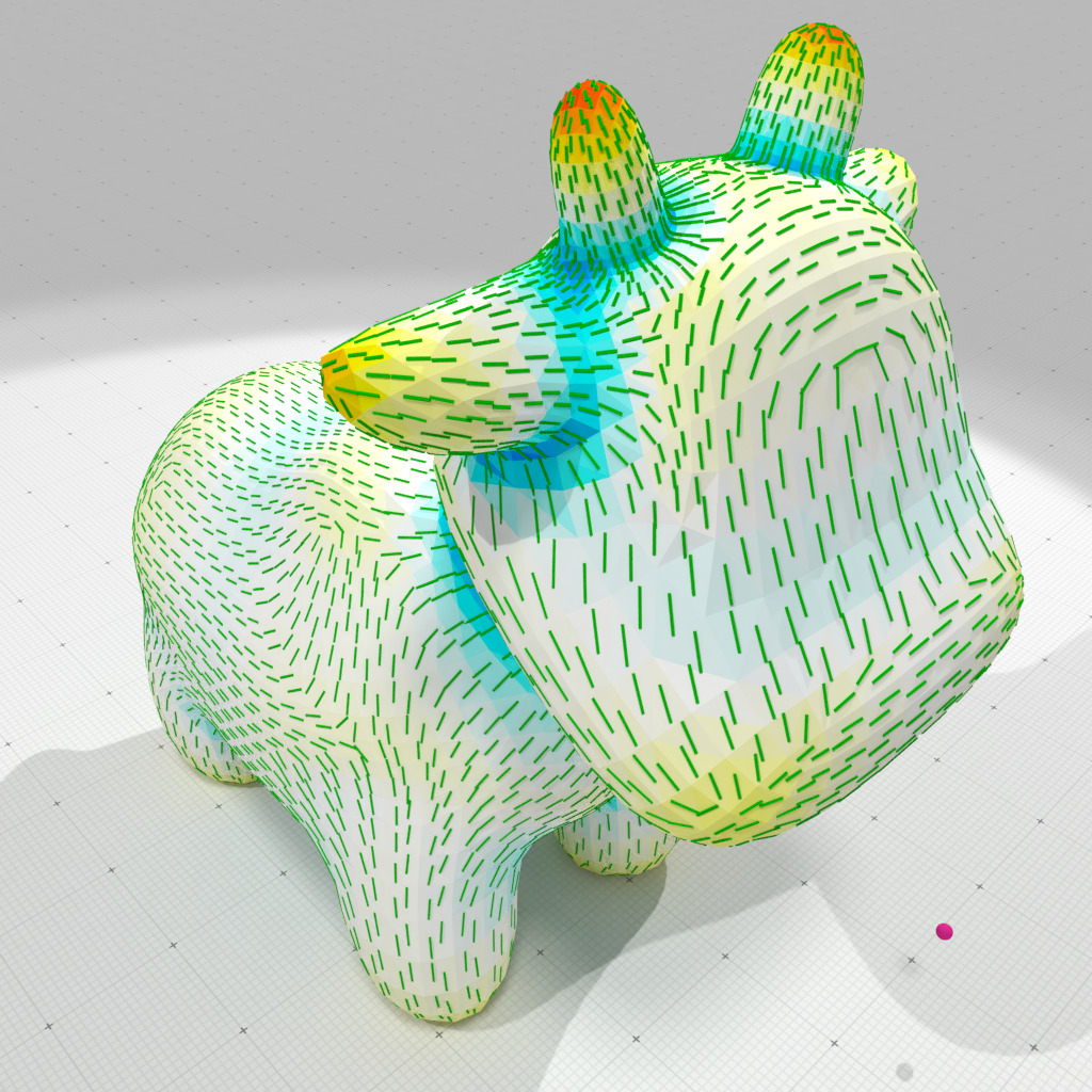
Interpolated corrected smallest principal curvature and direction, r=0.05 | 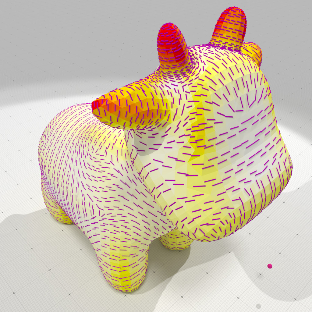
Interpolated corrected greatest principal curvature and direction, r=0.05 |
Corrected curvature measures on digital surfaces
It is difficult to estimate curvatures on digital surfaces, since they naturally have only very few normal directions. You may have a look at module Integral invariant curvature estimator 2D/3D to see a method that estimates such curvatures when the digital surface is the boundary of a volume of voxels.
Corrected Normal Currents are well adapted to digital surface geometric analysis. Indeed, we can have good estimates of the normal vector field of a digital surface (see ShortcutsGeometry), which will be used as the corrected normal vector field associated to the current.
As examples of digital surfaces, we show how to estimate curvatures on a digitization of polynomial surfaces, then on the boundary of a voxel object defined in VOL file.
CCNC and ICNC curvature measures on discretized polynomial surfaces
Examples geometry/meshes/digpoly-curvature-measures-cnc-3d.cpp and geometry/meshes/digpoly-curvature-measures-cnc-XY-3d.cpp show how to extract all curvature information from digitized polynomial surfaces.
We first read the polynomial definition and extracts the digital surface approximating the implicit surface at the given resolution.
We build a SurfaceMesh object that represents exactly the digital surface.
We build the Corrected Normal Current on this mesh, and use a digital estimator of normal vector (here convolved trivial normals) to set the corrected normal vector at each face or vertex, depending on the choice of the user.
The remaining of the code to estimate curvatures from measures is identical to above. You can obtain the following results:
Face-constant corrected mean curvature measure, r=1 | 
Face-constant corrected Gaussian curvature measure, r=1 | 
Face-constant corrected smallest principal curvature and direction, r=1 | 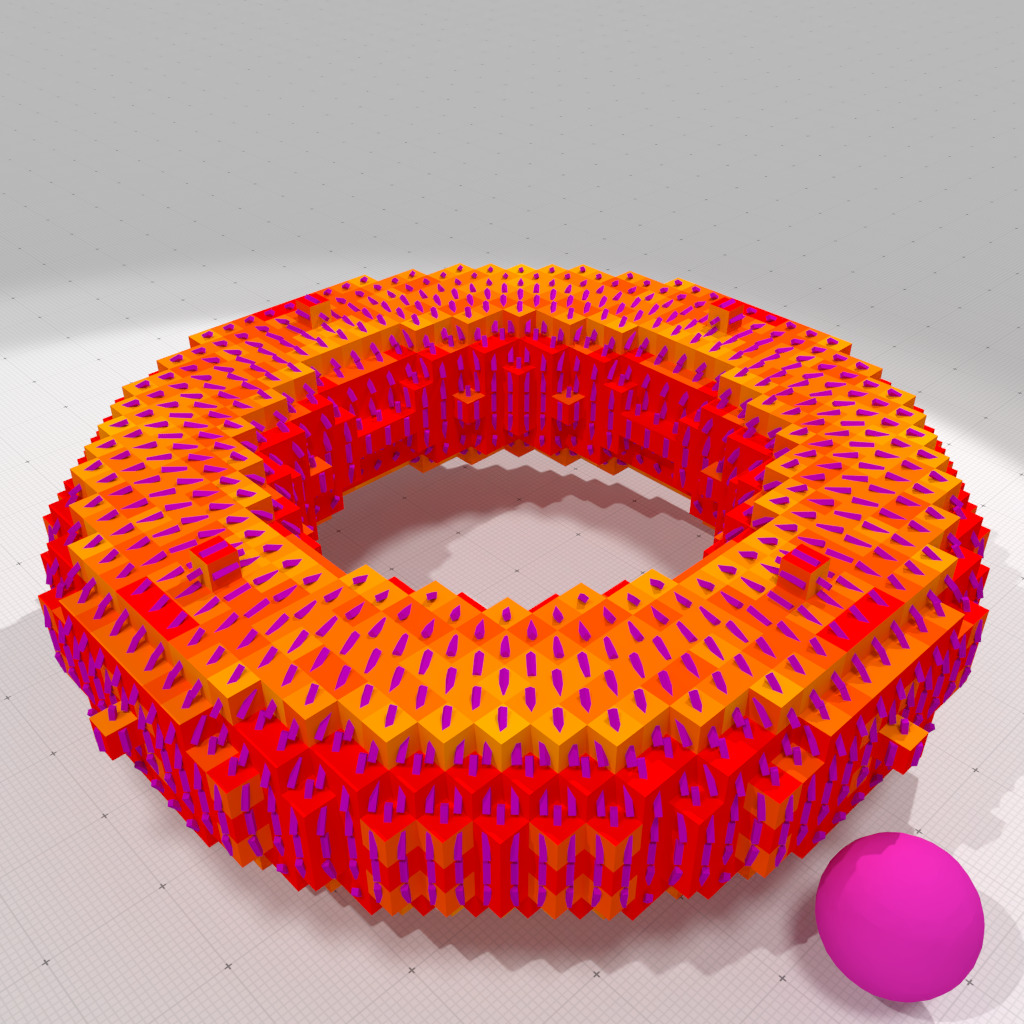
Face-constant corrected greatest principal curvature and direction, r=1 |
Vertex-interpolated corrected mean curvature measure, r=1 | 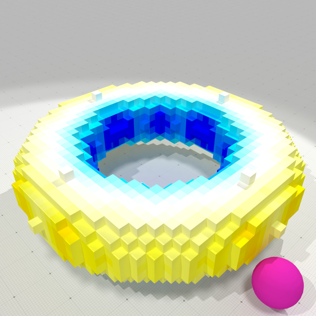
Vertex-interpolated corrected Gaussian curvature measure, r=1 | 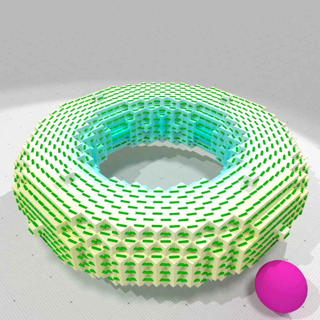
Vertex-interpolated corrected smallest principal curvature and direction, r=1 | 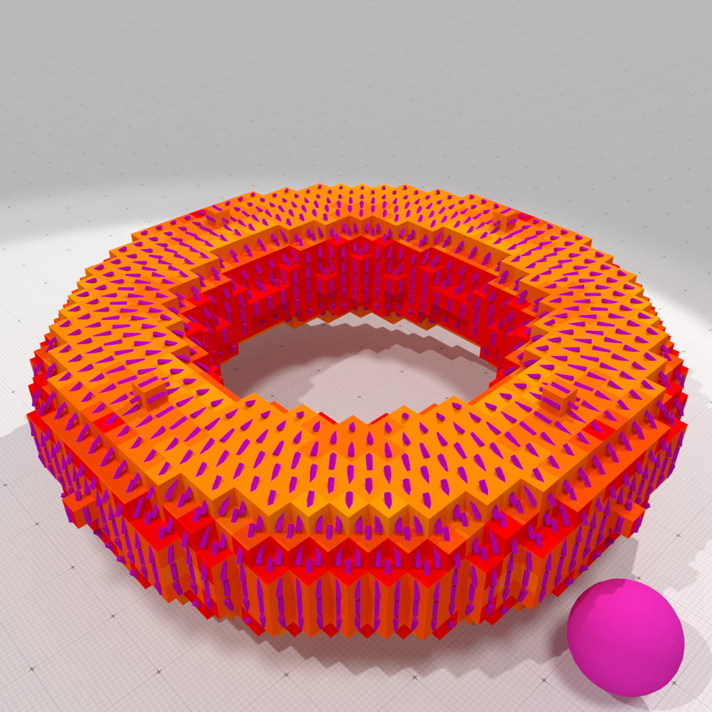
Vertex-interpolated corrected greatest principal curvature and direction, r=1 |
ICNC curvature measures on digital boundaries in VOL file
Examples geometry/meshes/vol-curvature-measures-icnc-3d.cpp and geometry/meshes/vol-curvature-measures-icnc-XY-3d.cpp show how to estimate curvatures on the boundary of a digital object.
We first read the VOL file and extracts the digital surface bounding the digital object.
We build a SurfaceMesh object that represents exactly the digital surface.
We build the Corrected Normal Current on this mesh, and use a digital estimator of the normal vectors (here convolved trivial normals) to set the corrected normal vector at each vertex.
The remaining of the code to estimate curvatures from measures is identical to above. We run the examples on "Al" vol file, which gives the following results.
Interpolated corrected mean curvature measure, r=2 | 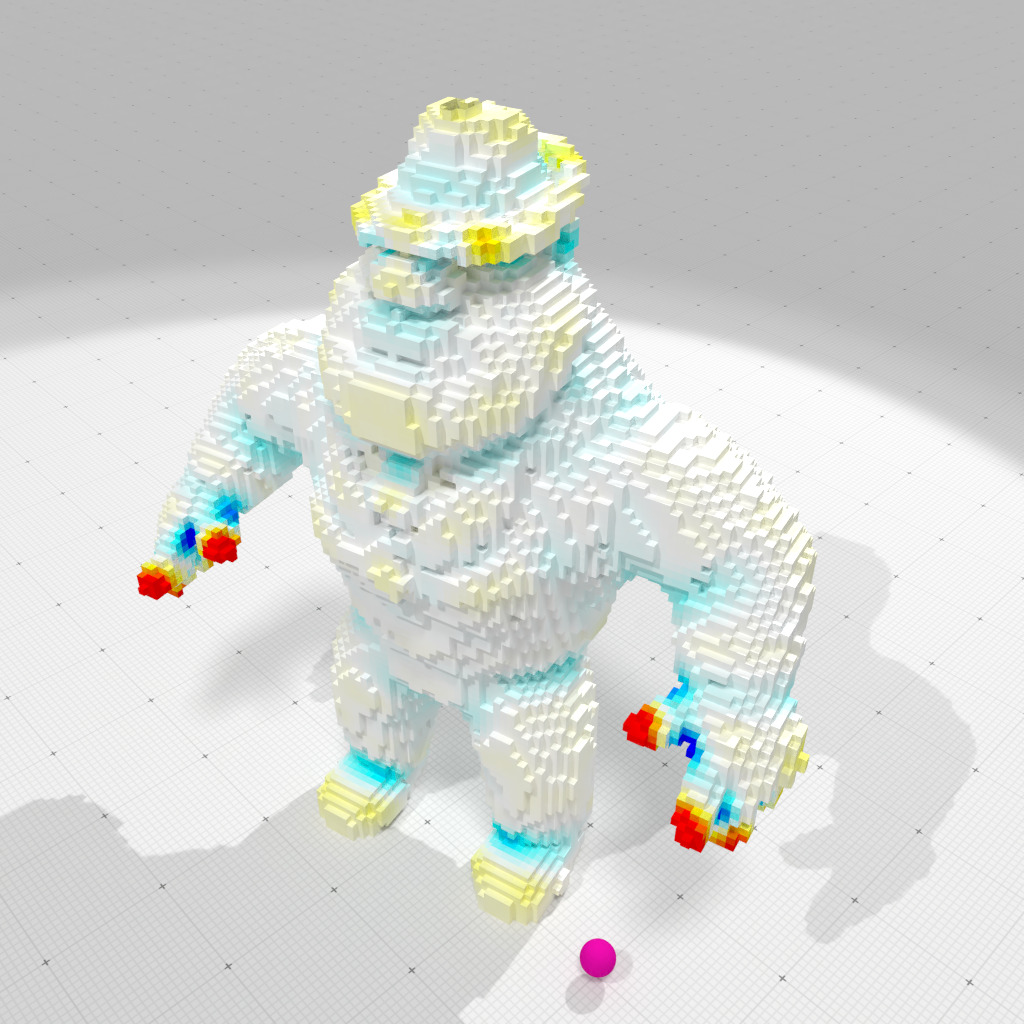
Interpolated corrected Gaussian curvature measure, r=2 | 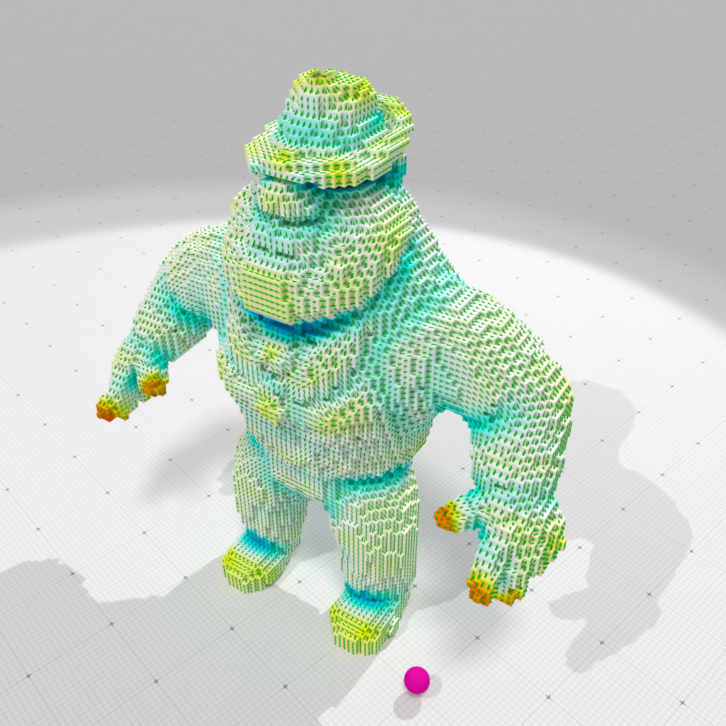
Interpolated corrected smallest principal curvature and direction, r=2 | 
Interpolated corrected greatest principal curvature and direction, r=2 |
Comparison between integral invariant and CNC curvature estimates on digital boundaries
We give below a few comparisons (in terms of accuracy and speed) between CNC curvature estimations and Integral Invariant (II) method (see Integral invariant curvature estimator 2D/3D). II method is a curvature estimation method specialized (and restricted) to boundaries of digital volumes (i.e. set of voxels). Therefore we compare their respective performance on digitizations of polynomial surfaces.
- Note
- We use example curvature-comparator-ii-cnc-3d.cpp to do the computations.
We run the tests on goursat polynomial surface, with digitization gridsteps \( h \in \{ 1, 0.5, 0.25, 0.125, 0.0625 \} \). Parameters are set up as follows:
- II method
- integration radius is \( R = 3h^{\frac{1}{3}} \), which is the standard parametrization,
- we test both mean curvature and Gaussian curvature estimations.
- CNC method
- corrected normal vector field is II normal vector estimation with also radius \( R = 3h^{\frac{1}{3}} \),
- measure radius for CNC is \( \rho = h^{\frac{1}{2}} \),
- either constant or interpolated CNC measures are computed,
- we test both mean curvature and Gaussian curvature estimations.
We plot below accuracy as a function of the digitization gridstep.
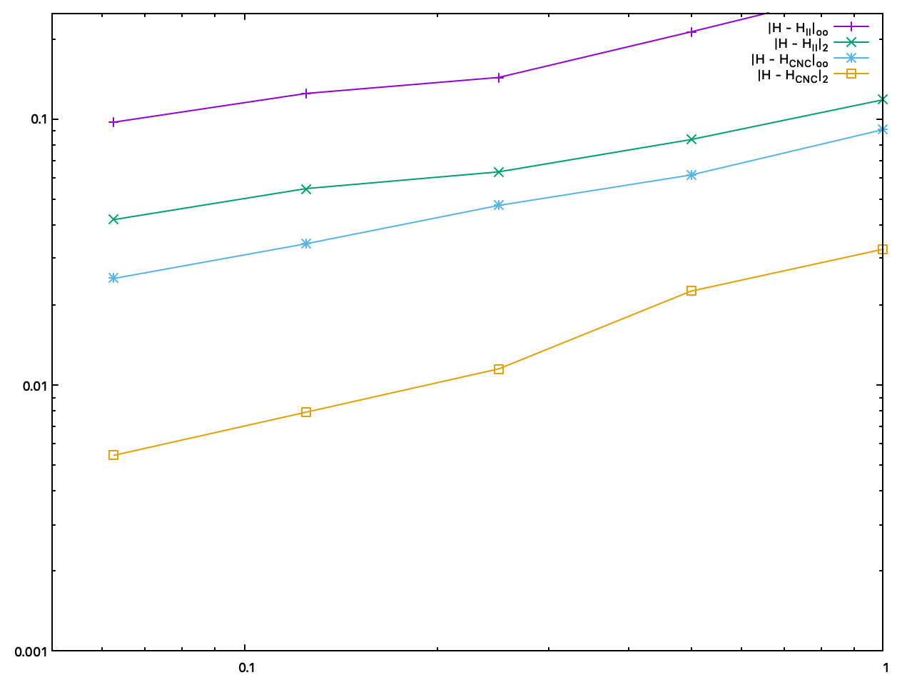
Accuracy comparison between II and constant CNC mean curvature estimates, as a function of the digitization gridstep | 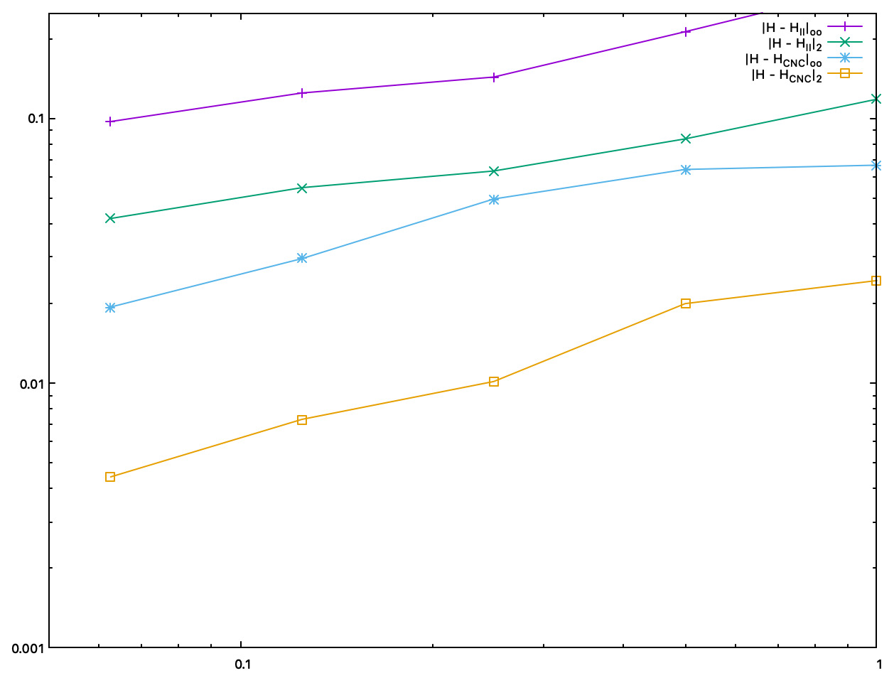
Accuracy comparison between II and interpolated CNC mean curvature estimates, as a function of the digitization gridstep | 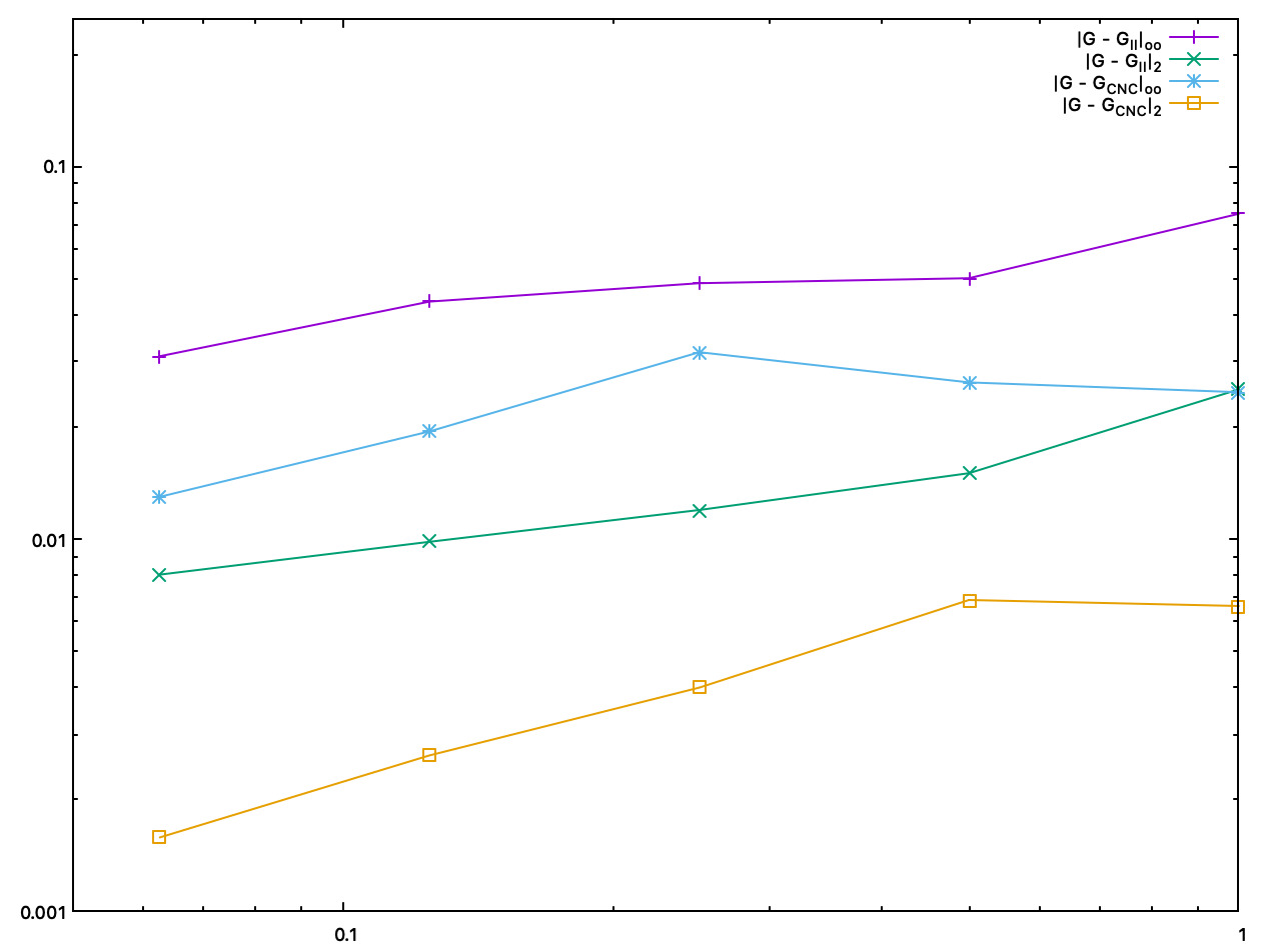
Accuracy comparison between II and interpolated CNC Gaussian curvature estimates, as a function of the digitization gridstep |
We plot below accuracy as a function of the computation time (in ms).
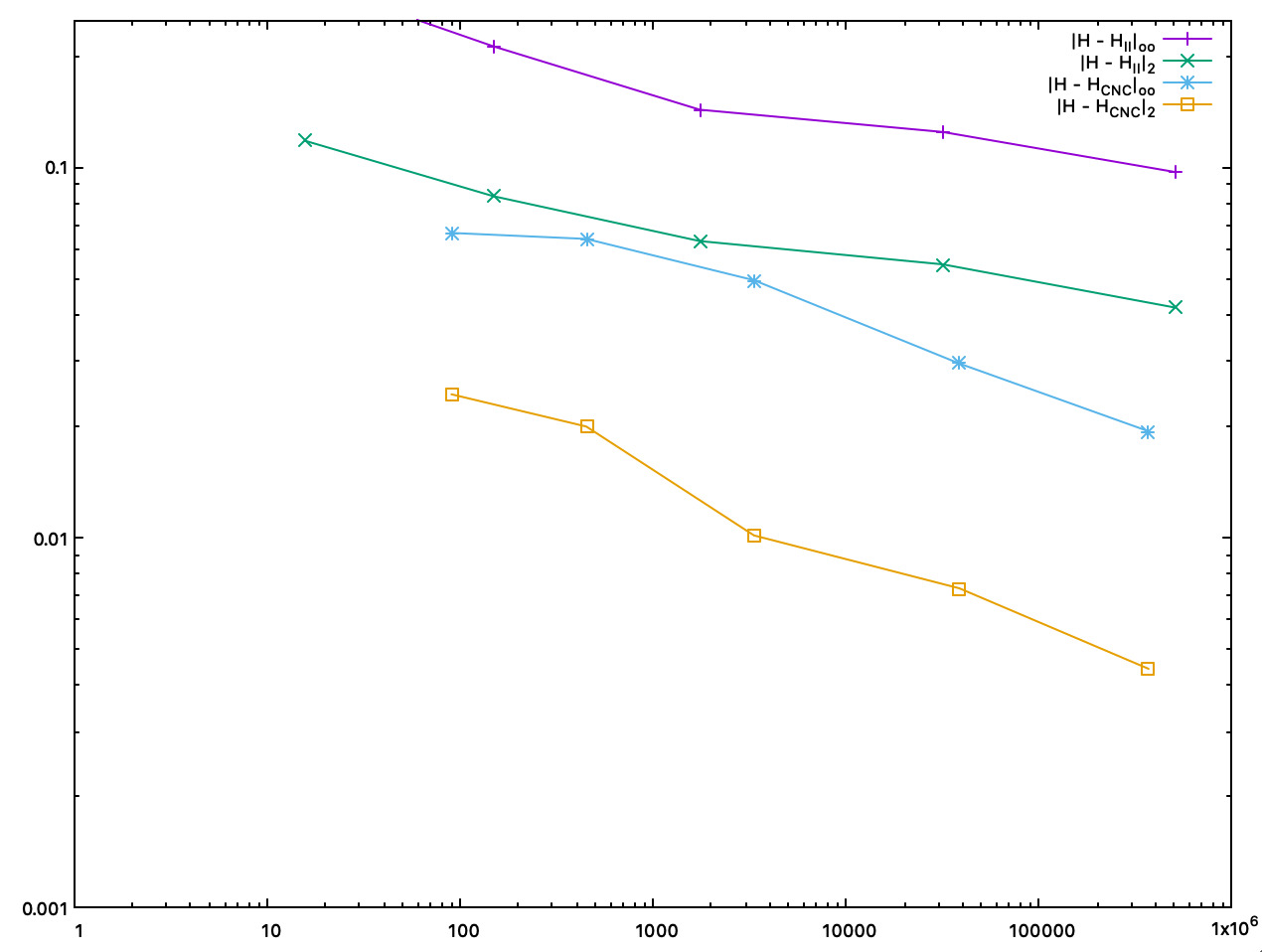
Accuracy comparison between II and interpolated CNC mean curvature estimates, as a function of the computation time (in ms) | 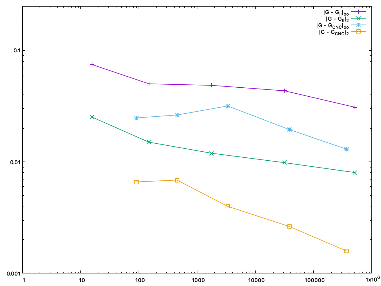
Accuracy comparison between II and interpolated CNC Gaussian curvature estimates, as a function of the computation time (in ms) |
| curvature estimator | number of surfels | error loo | error l2 | total time (ms) | normal estimation time (ms) |
|---|---|---|---|---|---|
| II mean curvature | 9510 | 0.212016 | 0.0835415 | 148 (mean+Gaussian) | |
| ICNC mean curvature | 9510 | 0.0640707 | 0.0199467 | 450 (mean+Gaussian) | 83 |
| II Gaussian curvature | 9510 | 0.0501252 | 0.0150247 | 148 (mean+Gaussian) | |
| ICNC Gaussian curvature | 9510 | 0.0263134 | 0.00686261 | 450 (mean+Gaussian) | 83 |
| II mean curvature | 151374 | 0.124552 | 0.0546997 | 31635 (mean+Gaussian) | |
| ICNC mean curvature | 151374 | 0.0295432 | 0.00730423 | 38582 (mean+Gaussian) | 19322 |
| II Gaussian curvature | 151374 | 0.0433595 | 0.00983477 | 31635 (mean+Gaussian) | |
| ICNC Gaussian curvature | 151374 | 0.0194384 | 0.00262745 | 38582 (mean+Gaussian) | 19322 |
- Note
- Both CNC curvature estimators are twice to five times more accurate than II curvature estimates. About speed, asymptotically, most of the time taken by CNC is for computing II normal vectors. Finally, as shown by pictures, CNC curvature estimates are much more stable than II curvature estimates, which tend to oscillate around the correct value.