Table of Contents
- Author(s) of this documentation:
- Pierre Gueth
Introduction
Discrete Exterior Calculus (DEC) provides a nice way to represent discrete scalar and vector fields, as well as linear vector analysis operators. It can be potentially applied to a large number of field theory problem, such as electrodynamics, thermodynamics or really any linear physics problem.
DEC extends efficiently continuous Riemannian geometry vector fields and differential forms to the discrete world. Discretization of differential forms induces a natural discretization of linear operators between them. This allows easy and fast resolution of linear problem over complex geometric objects.
DEC geometrical structure
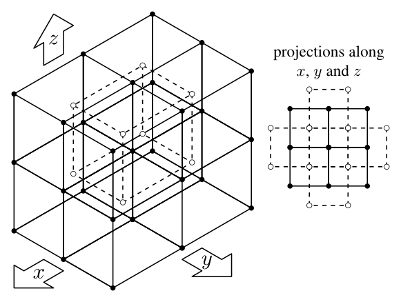
A DEC structure is composed of a primal and a dual k-cells sets which define the geometrical shape of the represented object. These sets are interleaved and are the dual of each others in the classical sense. Each pair of primal and dual k-cells holds primal and dual sizes used to define the Hodge duality operator. Associated primal k-cell and dual k'-cell don't have the same dimension. In general, \(k' = n - k\) where \(n\) is the dimension of the DEC structure.
- Note
- By definition 0-cell must have a primal size equals to 1 and n-cell must have dual size equals to 1.
Scalar field, k-form and vector field
DEC scalar field associate a scalar value to each 0-cells of the structure. DEC vector field associate an n dimensional quantity (a arrow for example) to each 0-cells of the structure.
DEC k differential forms, or k-forms for short, associate a scalar value to each primal or dual k-cells of the structure. They are the discrete extension of continuous differential forms defined in tensor calculus and Riemannian geometry to the discrete world. It important to remember that they can be used to transform k-vector into scalar fields and therefore form a base of k-vectors tangent bundles. Following this definition, the first example of k-forms are scalar fields, which are analogous to 0-forms. Discrete 1-forms, as their continuous counter part, can be constructed from vector fields to created "project along this vector field" operator. 1-forms are therefore linked to vector field and the DEC provides flat and sharp operators to transform one into the other. Higher order differential forms can be constructed from 0- and 1-forms through using wedge product to form complex structure such as metric tensor (n-form) or any other tensorial quantity.
Vector fields and k-forms come in both primal and dual flavors. Choosing duality has a small geometrical influence since primal and dual cells are slightly shifted, but most importantly this choice changes boundary conditions when solving linear DEC problem. See 1D Poisson resolution for an example.
Moreover k-forms and vector fields forms vector space as long as their duality and order is preserved. Two compatible fields or differential forms can therefore be added, subtracted or scaled through external multiplication.
Finally, it is important to note that non empty k-forms space exists only for \( 0 \leq k \leq n \). Knowing that base k-forms can be constructed for k 1-forms wedged together, it can be easily proven that if \( k > n \) the base vanishes due the antisymmetric nature of wedge product and the limited choice of linearly independent 1-forms. K-forms are represented using KForm class. Vector fields are represented using the VectorField class.
Discrete linear operators
Discretization of k-forms induces a discretization of linear operators between k-forms. An important statement of DEC is that any of those operators can be expressed easily using only two basic operations, Hodge duality operators \(\star\) and exterior derivative \(d\). Since k-forms vector spaces are in finite number, those operators are also in finite number. DEC defines two more operators : \(\sharp\) (sharp) transforms 1-forms into vector fields and \(\flat\) (flat) transforms vector fields into 1-forms. The following figure shows all available linear operators for a 3D structure, where TM (resp. TM') represents the primal (resp. dual) tangent bundle, the union of all tangent vector spaces generated by primal (resp. dual) vector fields. K-cells associated with k-forms are highlighted in red next to the k-form spaces. As for DEC objects, operators come also in both primal and dual flavor. Dual stuff have a prime and primal stuff stay pristine. Linear operators between k-forms are represented by LinearOperator class.
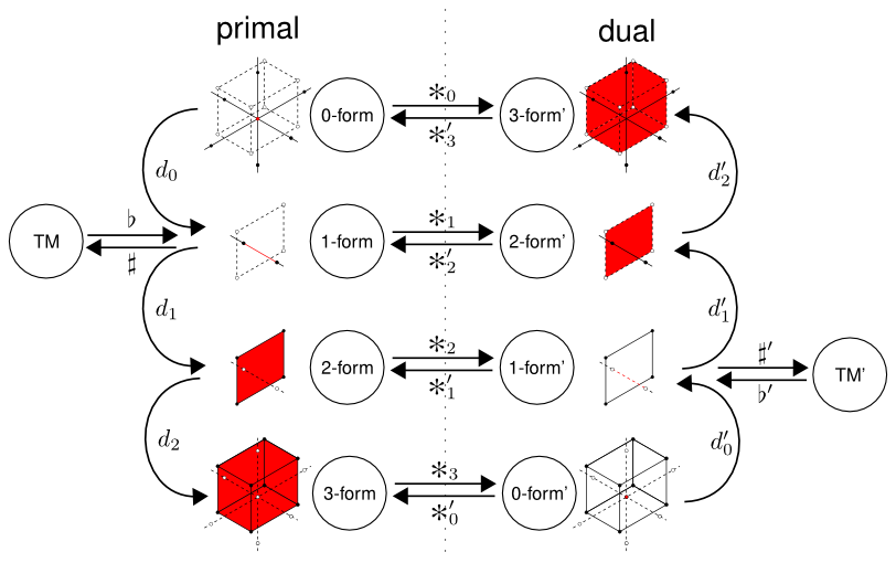
Hodge duality operator
Intuitively, one can think of Hodge duality operator as orthogonal complement operators on k-cells. Wedging any k-cells with its orthogonal complement always forms the volume form (single n-form base). They take care of size ratio and orientation change between primal and dual meshes. \(\star_k\) (resp. \(\star_k'\)) take primal (resp. dual) k-forms as input and create dual (resp. primal) (n-k)-forms. Hodge operators are defined by their action on a value of a discrete k-form \(x\) at a k-cell \(\sigma\).
\[ \star x ( \star\sigma ) = \frac{|\star\sigma|}{|\sigma|} x ( \sigma )\]
where \(|\sigma|\) is the size of \(\sigma\). Applying \(\star\) twice to a k-form \(x\) will give \(x\) back up to sign given by the following equation.
\[ \star \star x = -1^{(n-k)k} x \]
Most of the time applying \(\star\) twice is the same as applying an identity operator. The first two Hodge operators switch k-form sign is for \(n=2\) and \(k=1\) : taking twice the orthogonal of edge in a 2D structure result in a sign flip of the corresponding 1-form. From the equation above, one can show that 4 \(\star\) always contract to identity.
\[ \star \star \star \star x = x \]
Primal Hodge operators \(\star_k\) and dual Hodge operators \(\star_k'\)) are generated using DiscreteExteriorCalculus.hodge with k as the first template parameter and duality as the second template parameter. See wikipedia page for more details.
Exterior derivative
Exterior derivative operators are the second kind of basic operator on which DEC is built. Exterior derivatives take k-forms as inputs and create (k+1)-forms. Input and output forms keep the same duality. As all derivative operators, \(d\) follow the Leibniz rule for derivative of a product of k-forms.
\[ d ( x \wedge y ) = d x \wedge y + (-1)^k x \wedge d y \]
where x is a k-form and y is a k'-form with the same duality. Applying any exterior derivative twice always vanishes.
\[ d d x = 0 \]
This rules out many buildable complex linear operators as one has to switch duality every time a derivative is applied. In the DEC package, exterior derivative operators are generated using DiscreteExteriorCalculus.derivative with input k-form order as the first template parameter and duality as the second template parameter. See wikipedia page for more details.
Antiderivative
Antiderivative operators are shorthand operators that appear in many DEC problems. They take k-forms as inputs and create (k-1)-forms. Input and output forms keep the same duality. Here is the definition of \(\delta\), the antiderivative acting on k-forms.
\[ \delta = \star' d' \star \]
In the DEC package, antiderivative operators are generated using DiscreteExteriorCalculus.antiderivative. As for \(d\), applying any antiderivative twice vanishes.
\[ \delta \delta x = 0 \]
Sharp and flat
Sharp \(\sharp\) and flat \(\flat\), called musical isomorphisms in [44], transform 1-form into vector field and the other way around. In the continuous world, these two operators cancel each other exactly.
\[ (x ^\sharp) ^\flat = x \]
\[ (y ^\flat) ^\sharp = y \]
where \(x\) is a 1-form and \(y\) is a vector field of the same duality. The bijectivity of these operators is slightly altered by the discretization. Therefore application of sharp and flat will induce a small divergence from the origin. This is especially visible along borders of the structure. Contrary to Hodge operators and exterior derivative, sharp and flat operators don't exist as stand alone object, but rather get applied by the DEC structure directly through DiscreteExteriorCalculus.sharp and DiscreteExteriorCalculus.flat.
Classical vector analysis
Classical vector analysis operators such as gradient \(\nabla\), divergence \(\nabla\cdot\), curl \(\nabla\wedge\) and Laplace operator \(\Delta\) can be expressed with basic DEC operators, \(\star\), \(d\), \(\sharp\) and \(\flat\).
\[\nabla x = ( d x )^\sharp \]
\[\nabla\cdot x = \star d \star x^\flat = \delta x \]
\[\nabla\wedge x = ( \star d x^\flat )^\sharp \]
\[\Delta x = \star d \star d x = \delta d x \]
Note that each basic operators changes with the dimension of the structure \(n\) and duality of the input k-form vector space.
Laplace operators
In order to find the right operators to use, one could draw a figure similar to Figure two. Using this figure together with the definition of vector analysis operators provided in the above section, the order and duality of each operator become easy to figure out. For example, one can easily figure out the precise definition of the primal Laplace operator \(\Delta\) and the dual Laplace operator \(\Delta'\) in 3D dimension. Paths taken by those operators are highlighted in Figure three. \(\Delta\) can be expressed using derivative and antiderivative.
\[ \Delta = \star_3' d_2' \star_1 d_0 = \delta_1 d_0 \]
\[ \Delta' = \star_3 d_2 \star_1' d_0'= \delta_1' d_0' \]
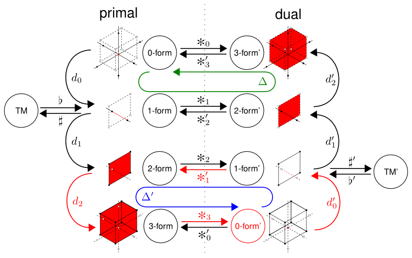
If the dimension of the DEC structure changes, the definition of the primal Laplace operator changes slightly. For example, here is the definition of the primal Laplace operator in 2D. Note that the expression using antiderivative do not change.
\[ \Delta = \star_2' d_1' \star_1 d_0 = \delta_1 d_0 \]
Note that DiscreteExteriorCalculus provides DiscreteExteriorCalculus.laplace to conveniently compute Laplace operators. Of course, one could still built Laplace operator of basic Hodge and derivative (see 2D Helmoltz decomposition).
DEC linear problem
Using the DEC package, one can solve any equation of the type:
\[ f(x) = y \]
where \(x\) and \(y\) are k-forms, with potentially different orders and dualities, and \(f\) is a linear operator between k-forms. One can create linear operators by manually filling LinearOperator.myContainer, but it's often easier to combine derivative \(d\) and duality operators \(\star\) computed by DiscreteExteriorCalculus.derivative and DiscreteExteriorCalculus.hodge.
Recall that \(\flat\) and \(\sharp\) are operators that turn a vector field into a 1-form and the other way around. Those operators are linear but do not transform k-forms into k-forms and therefore can't be represented by LinearOperator. However DiscreteExteriorCalculus allows us to apply those transformations on associated k-forms and vector fields, namely DiscreteExteriorCalculus.flat and DiscreteExteriorCalculus.sharp. These operators are cached in the DiscreteExteriorCalculus object and support intense load, as Hodge and derivative operators do. We chose to disable \(\flat\) and \(\sharp\) representation because the quantity of information stored in the associated 1-form is always bigger than the quantity of information stored in the vector field.
Further reading
- Keenan Crane SIGGRAPH lecture 2013 "Geometry processing using DEC" github repository [44]
- Mathieu Desbrun article on discrete exterior calculus [49]
- Digital foam presentation with an introduction to DEC in the second section pdf
Hands on the DEC package
This section provides an overview on structures and classes that compose the DEC package. All snippets are taken from exampleDiscreteExteriorCalculusUsage.cpp. Here is a typical list of headers needed to use the DEC package.
Main DEC object creation
In this package, the main DEC object is DiscreteExteriorCalculus. The first template parameter is the dimension of the embedded structure one wants to represent. The second template parameter is the dimension of the ambient space in which the structure in embedded. For obvious reasons, the ambient dimension must be equal or greater than the embedded dimension. The ambient dimension is used internally by DiscreteExteriorCalculus.myKSpace and therefore is the maximum dimension of cells and points used to fill the DEC object. The third template parameter is a linear algebra backend used internally to specify containers and solvers. By now, there is only one available backend: EigenLinearAlgebraBackend. For example, here is a snippet that define a working two dimensional DEC object embedded in a two dimensional ambient space along with the corresponding factory type.
The DiscreteExteriorCalculus provides a default constructor that initializes an empty structure, ready to be filled with DiscreteExteriorCalculus::SCell through the DiscreteExteriorCalculus.insertSCell member. DiscreteExteriorCalculus objects can also be created using the DiscreteExteriorCalculusFactory factory. DiscreteExteriorCalculusFactory::createFromDigitalSet static member inserts each point of a digital set as a primal n-cell in the structure and then fills in-between k-cells to glue all n-cells together. DiscreteExteriorCalculusFactory::createFromNSCells static member creates embedded structures. See Embedding n-dimensional DEC structures into m-dimensional space for a discussion about manifold embedding. Borders can be added or removed from the generated structure using the add_border boolean to enforce various boundary condition. Dual k-cells are created automatically. Note that the structure can be altered after creation to adjust small details or created completely manually via calls to DiscreteExteriorCalculus.insertSCell and DiscreteExteriorCalculus.eraseCell.
- Note
- Internal indexes should be reset by calling DiscreteExteriorCalculus.updateIndexes after any call to DiscreteExteriorCalculus.insertSCell or DiscreteExteriorCalculus.eraseCell and before doing anything else with the structure. This includes instantiation of any KForm, VectorField or LinearOperator as well as any type of output and size computation. DiscreteExteriorCalculus created by DiscreteExteriorCalculusFactory have valid indexes and can be used as it is.
This snippet shows how to create a DEC structure. The first call to DiscreteExteriorCalculus.eraseCell removes the primal n-cell located of the right of the structure. The associated dual 0-cell is destroyed automatically. Note that n-cells are created using KhalimskySpaceND.sSpel, and that coordinates of such cells are given in the same system as points from the input set. The second call removes a primal 1-cell and opens the hole created by the first call. Here coordinates are given in the KhalimskySpaceND signed cell frame of reference. To finalize the structure, a call to DiscreteExteriorCalculus.updateIndexes is performed.
Note moreover that in DEC, positive 1-cells are oriented is the opposite direction of increasing coordinates.
If you want to have border-less structure, simply reset the add_border boolean. See Border definition for a discussion about border definition. The second call to DiscreteExteriorCalculus.eraseCell isn't needed anymore since the edge was not inserted in the first place.
Sometime one doesn't want to create DEC structure from higher order cells using the set factory of DiscreteExteriorCalculusFactory. It is possible to insert cells manually into the DEC structure using DiscreteExteriorCalculus.insertSCell. Inserting a new cell invalidate all previously created k-forms, linear operators and vector fields. Therefore the DEC structure shouldn't be modified once DEC operators are created.
KForm and VectorField manipulation
K-forms are represented by the KForm templated class and vector field are represented by the VectorField templated class. Note that DiscreteExteriorCalculus provides handy typedef of common k-forms and vector field, such as DiscreteExteriorCalculus::PrimalForm0, DiscreteExteriorCalculus::DualForm2, DiscreteExteriorCalculus::PrimalVectorField and DiscreteExteriorCalculus::DualVectorField. Once a k-form is created, its actual values can by accessed through KForm.myContainer. Cell indexes can be retrieved from cells using DiscreteExteriorCalculus.getSCell and cell can be retrieved from cells using DiscreteExteriorCalculus.getSCell.
Convenience members KForm.length, VectorField.length, KForm.getSCell and VectorField.getSCell can be used to traverse structures easily. Here is a example snippet that compute a Euclidean distance map (scalar field) on the structure defined above.

K-forms, as vector field, can be scaled, added and subtracted using standard cpp operators.
In the snippet, we compute the primal gradient of the previous scalar field using formula from Classical vector analysis. Convenience linear operator DiscreteExteriorCalculus::DualDerivative0 is used.
Flat and sharp operators are applied to test the property presented in Sharp and flat. Original vector field and its dual sharped version differ slightly along the border of the structure. See bottom right part on the inner hole for example.
The orthogonality of the Hodge operator is demonstrated here, as we compute the dual of the gradient vector field described above. One can see that primal of dual vector fields are always locally orthogonal everywhere.
DEC linear solver
If your problem can be described as a DEC linear problem, DiscreteExteriorCalculusSolver can be used to solve it.
The solving method used is provided as the second template parameter of DiscreteExteriorCalculusSolver. It depends on the linear algebra backend you pass as second template argument in the definition of DiscreteExteriorCalculus. Usually some linear solvers are provided in the linear algebra backend itself, but you can create your own as long as it models the CLinearAlgebraSolver concept.
Using Eigen detected when building the project, you can use any solver provided in the EigenSupport.h header. It is recommended to use the EigenLinearAlgebraBackend since it is fast and provide a lot of linear solvers.
Once the DEC solver is created, the linear operator \(f\) must be passed via DiscreteExteriorCalculusSolver.compute. Depending on the linear solver used, this will factorize the problem or do precomputation on the linear operator. This speed up the resolution of problems that share the same linear operator. Input k-form \(y\) is passed to the solver via DiscreteExteriorCalculusSolver.solve which return the solution k-form \(x\). If the resolution was successful, then DiscreteExteriorCalculusSolver.isValid will return true. If there was a problem, it can be further investigated by direct access to the linear algebra solver DiscreteExteriorCalculusSolver.solver.
Choosing the right solver for the right problem has a direct impact on overall performances. The EigenLinearAlgebraBackend provide wrapper for all linear algebra solvers included in the Eigen library. This documentation page provides a nice summary of wrappable solvers along with their main traits.
Resolution of Poisson equation and Helmoltz decomposition are provided as example.