DGtal  1.4.beta
Poisson problem
Author(s) of this documentation:
Pierre Gueth

Poisson equation

The Poisson equation can be written as:

\[ \Delta \phi = f \]

where \(\Delta\) is the Laplace operator, \(\phi\) the solution of the problem and \(f\) the input of the problem. The Poisson equation can be viewed as the heat equation when steady state is reached. \(f\) is then the constant spatial heating power applied to the structure and \(\phi\) is the temperature reached in steady state (up to a spatial constant). Here we choose \(f\) to be a Dirac delta function \(\delta\) to simulate a punctual heating on the structure.

Depending on border conditions, \(\Delta\) may have some null eigenvalues. In order to make it solvable, we use a regularized version of the Laplace operator \(\Delta_\mathrm{reg}\), defined below

\[ \Delta_\mathrm{reg} = \Delta + \lambda I \]

where \(I\) is the identity operator and \(\lambda\) is the regularization scalar, chosen small with respect to \(\Delta\) eigenvalues. Linear regularized solution are the same solution as least square problem solution of the non regularized problem. \(I\) is generated using DiscreteExteriorCalculus.identity.

One can use the general Laplace operator definition.

\[ \Delta = \star d \star d = \delta d \]

However, for convenience DiscreteExteriorCalculus provides a method to get the Laplace operator directly.

1D Poisson resolution

In this example, we create an 1D linear structure embedded in a 2D space and we solve a non regularized Poisson equation on this structure.

Boundary conditions effect are illustrated for the two classical boundary conditions.

  • Neumann boundary condition forces the derivative to be null along the border of the structure. Here, this means that heat can't flow out the start and the end of the linear structure.
  • Dirichlet boundary condition connects borders of the structure to null potential. With our heat analogy, this means that the start and the end of the linear structure are connected to thermostat, which are given the null temperature.

Boundary conditions are changed from Neumann to Dirichlet conditions by adding dangling 1-cells at the beginning and at the end of the structure. Snippets are taken from testLinearStructure.cpp.

Neumann boundary condition

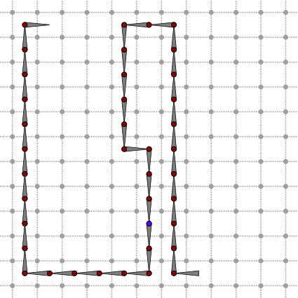
First, an empty calculus structure is created and, using simple for loops, it is filled with some 0-cells and 1-cells to from a linear structure. When filled manually with DiscreteExteriorCalculus.insertSCell, one can pass the primal and dual sizes of each cell which default to 1. Temperature nodes are associated primal 0-cells. Note that to enforce Neumann boundary conditions, the linear structure has to end with 0-cells. Moreover some 1-cells are inserted as negative cells to match their orientation with the orientation of the linear structure.

typedef DiscreteExteriorCalculus<1, 2, EigenLinearAlgebraBackend> Calculus;
SCells cells;
// fill cells container
{
const Calculus::KSpace kspace;
for (int kk=20; kk>0; kk--) cells.push_back( kspace.sCell(Point(0,kk), kk%2 != 0 ? Calculus::KSpace::NEG : Calculus::KSpace::POS) );
for (int kk=0; kk<10; kk++) cells.push_back( kspace.sCell(Point(kk,0)) );
for (int kk=0; kk<10; kk++) cells.push_back( kspace.sCell(Point(10,kk)) );
cells.push_back( kspace.sCell(Point(10,10)) );
cells.push_back( kspace.sCell(Point(9,10), Calculus::KSpace::NEG) );
for (int kk=10; kk<20; kk++) cells.push_back( kspace.sCell(Point(8,kk)) );
for (int kk=8; kk<12; kk++) cells.push_back( kspace.sCell(Point(kk,20)) );
for (int kk=20; kk>0; kk--) cells.push_back( kspace.sCell(Point(12,kk), kk%2 != 0 ? Calculus::KSpace::NEG : Calculus::KSpace::POS) );
cells.push_back( kspace.sCell(Point(12,0)) );
}
// fill calculus
const Domain domain(Point(-1,-1), Point(10,10));
// create DEC structure
Calculus calculus;
calculus.initKSpace<Domain>(domain);
for (SCells::const_iterator ci=cells.begin(), ce=cells.end(); ci!=ce; ci++) calculus.insertSCell( *ci );
calculus.updateIndexes();
KSpace::SCells SCells
Definition: StdDefs.h:82
MyPointD Point
Definition: testClone2.cpp:383
Domain domain
HyperRectDomain< Space > Domain

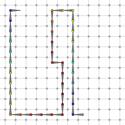
The input heat vector \(f\), which is a primal 0-form in the DEC formulation, is then created and is given values of a Dirac pulse shifted at the right position.

Calculus::Cell dirac_cell = calculus.myKSpace.uCell(Point(10,4));
Calculus::PrimalForm0 dirac = Calculus::PrimalForm0::dirac(calculus, dirac_cell);
KSpace::Cell Cell
Linear structure with Neumann boundary conditions. The input dirac 0-form is displayed, the blue 0-cell is where the non zero point of the Dirac is located.

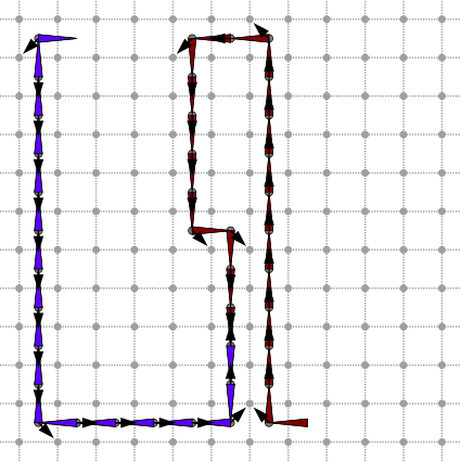
The primal non regularized Laplace operator \(\Delta\) is generated using DiscreteExteriorCalculus.laplace. The primal exterior derivative from 0-form to 1-form will be used to compute the gradient solution.

const Calculus::PrimalIdentity0 laplace = calculus.laplace<PRIMAL>();
@ PRIMAL
Definition: Duality.h:61

Now the problem is fully defined and there one thing left to do: solving it. The resolution is done by DiscreteExteriorCalculusSolver. This class takes the actual linear solver used as the second template parameter. Any class that validates the CLinearAlgebraSolver concept can be wrapped by DiscreteExteriorCalculusSolver. If DGtal was compiled with eigen support enabled as described in DEC linear solver, some solvers will be available in the EigenLinearAlgebraBackend. Here, we will use the EigenLinearAlgebraBackend::SolverSparseQR solver. Once created the solver is given the operator using DiscreteExteriorCalculusSolver.compute. The input dirac 0-form is passed to DiscreteExteriorCalculusSolver.solve, which return the solution of the problem.

typedef EigenLinearAlgebraBackend::SolverSparseQR LinearAlgebraSolver;
typedef DiscreteExteriorCalculusSolver<Calculus, LinearAlgebraSolver, 0, PRIMAL, 0, PRIMAL> Solver;
Solver solver;
solver.compute(laplace);
Calculus::PrimalForm0 solved_solution = solver.solve(dirac);
Eigen::SparseQR< SparseMatrix, Eigen::COLAMDOrdering< SparseMatrix::Index > > SolverSparseQR
Definition: EigenSupport.h:110

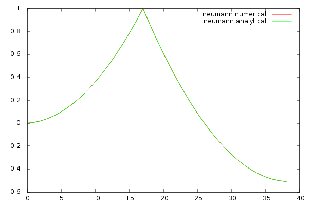
Since the dirac input is null everywhere except at a single point, this means that the second derivative of the solution is null everywhere except at the dirac position. An analytic form can be expressed as a continuous piece-wise quadratic function. Numerical values of the solution fit analytic values with at least a relative precision of 1e-5.

Linear structure with Neumann boundary conditions. Solution 0-form is displayed.
Linear structure with Neumann boundary conditions. Gradient 1-form and vector field are displayed.
Numerical values computed using the solver and analytic solution for the Neumann problem.

Dirichlet boundary condition

Dirichlet boundary condition fixes value of 0-forms to zero along borders of the structure. Two dangling 1-cells are added at each end of the Neumann structure to switch to Dirichlet boundary condition. Since those 1-cells are not connected to a 0-cell on one of their border, this will simulate the presence of zero-valued 0-cell in those places through enforcing Dirichlet boundary conditions.

calculus.insertSCell( calculus.myKSpace.sCell(Point(13,0)) );
calculus.insertSCell( calculus.myKSpace.sCell(Point(1,20), Calculus::KSpace::NEG) );
calculus.updateIndexes();

The input Dirac can be used as in the Neumann case since no 0-cells has been added to the structure.

Linear structure with Dirichlet boundary conditions. The input dirac 0-form is displayed, the blue 0-cell is where the non zero point is located. Two dangling edges were added at each ends of the structure.

Laplace operator needs to be rebuild, even if the code doesn't change.

const Calculus::PrimalIdentity0 laplace = calculus.laplace<PRIMAL>();

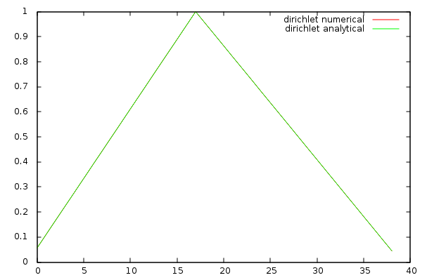
Solving the problem is achieved by using the same code as for the Neumann case. This time the analytic solution is piece-wise linear and take a constant null value at the border of the structure, as expect from the Dirichlet boundary condition.

typedef EigenLinearAlgebraBackend::SolverSparseQR LinearAlgebraSolver;
typedef DiscreteExteriorCalculusSolver<Calculus, LinearAlgebraSolver, 0, PRIMAL, 0, PRIMAL> Solver;
Solver solver;
solver.compute(laplace);
Calculus::PrimalForm0 solved_solution = solver.solve(dirac);

Numerical values of the solution fit analytic values with at least a relative precision of 1e-5.

Linear structure with Dirichlet boundary conditions. Solution 0-form is displayed.
Linear structure with Dirichlet boundary conditions. Gradient 1-form and vector field are displayed.
Numerical and analytic solution for the Dirichlet problem.

2D Poisson problem

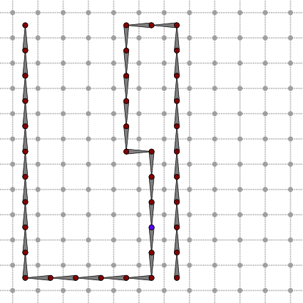
In this example, we create a 2D ring structure and we solve a regularized Poisson equation on this structure. Snippets are taken from exampleDiscreteExteriorCalculusSolve.cpp. First the structure is created from a digital set.

typedef DiscreteExteriorCalculus<2, 2, EigenLinearAlgebraBackend> Calculus;
typedef DiscreteExteriorCalculusFactory<EigenLinearAlgebraBackend> CalculusFactory;
Calculus calculus = CalculusFactory::createFromDigitalSet(generateRingSet(domain));

Then we compute the dual regularized Laplace operator with \(\lambda = 0.01 \).

Calculus::DualIdentity0 laplace = calculus.laplace<DUAL>() + 0.01 * calculus.identity<0, DUAL>();
@ DUAL
Definition: Duality.h:62

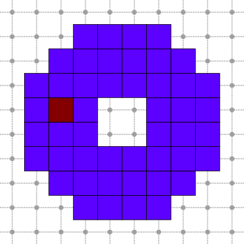
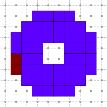
Input k-form \(y\) is a Dirac delta positioned on the dual 0-cell at coordinates \((2,5)\). DiscreteExteriorCalculus.getIndex return the index of the dual 0-form container associated with the dirac position cell.

Calculus::DualForm0 dirac(calculus);
dirac.myContainer(calculus.getCellIndex( calculus.myKSpace.uSpel(Z2i::Point(2,5))) ) = 1;
Space::Point Point
Definition: StdDefs.h:95

The following illustration represents the dual of the input. Hence, since we have specified a dirac on "dual 0-cell", its primal representation attaches information to (primal) 2-cells.

Input dual 0-form.

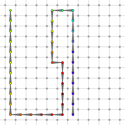
We try to solve the problem using EigenLinearAlgebraBackend::SolverSimplicialLLT, but DiscreteExteriorCalculusSolver.isValid reports an error. Underlying linear algebra solver DiscreteExteriorCalculusSolver.solver.info reports a numerical_error.

typedef DiscreteExteriorCalculusSolver<Calculus, LinearAlgebraSolver, 0, DUAL, 0, DUAL> Solver;
Solver solver;
solver.compute(laplace);
Calculus::DualForm0 solution = solver.solve(dirac);
trace.info() << solver.isValid() << " " << solver.myLinearAlgebraSolver.info() << endl;
std::ostream & info()
Trace trace
Definition: Common.h:153
Eigen::SimplicialLLT< SparseMatrix > SolverSimplicialLLT
Solvers on sparse matrices.
Definition: EigenSupport.h:105
Poisson problem solution computed with simplicial LLT solver. Solver reports a numerical error.

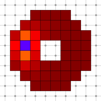
Since the first solver failed, let's use another one: EigenLinearAlgebraBackend::SolverSimplicialLDLT for example. This time DiscreteExteriorCalculusSolver.isValid is true after computing problem solution and the solution dual 0-form contains the solution of the problem.

typedef DiscreteExteriorCalculusSolver<Calculus, LinearAlgebraSolver, 0, DUAL, 0, DUAL> Solver;
Solver solver;
solver.compute(laplace);
Calculus::DualForm0 solution = solver.solve(dirac);
trace.info() << solver.isValid() << " " << solver.myLinearAlgebraSolver.info() << endl;
Eigen::SimplicialLDLT< SparseMatrix > SolverSimplicialLDLT
Definition: EigenSupport.h:106
Poisson problem solution computed with simplicial LDLT solver. Solver solution is valid.

Embedded 2D Poisson problem

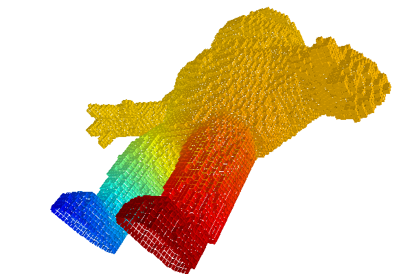
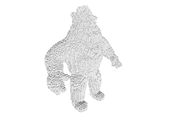
In this example, we create an embedded 2D structure from a DigitalSurface and we solve a dual Poisson equation with Neumann boundaries condition. Snippets are taken from exampleDECSurface.cpp.

First we load the Alcapone image and extract its boundary surface. Note that the Khalimsky space domain opens the surface under the feet of Alcapone.

const DGtal::Z3i::Domain domain = image.domain();
trace.info() << "domain=" << domain << endl;
typedef FalseOutsideDomain<Image, DGtal::Z3i::Domain> ImageExtended;
const ImageExtended image_extended(image, domain);
kspace.init(domain.lowerBound(), domain.upperBound()+DGtal::Z3i::Point(0,0,1), true);
typedef DGtal::SurfelAdjacency<3> SurfelAdjacency;
const SurfelAdjacency surfel_adjacency(true);
const DigitalSurfaceContainer digital_surface_container(kspace, image_extended, surfel_adjacency, cell_bel);
const DigitalSurface digital_surface(digital_surface_container);
Aim: Represents a set of n-1-cells in a nD space, together with adjacency relation between these cell...
Aim: This class is a model of CCellularGridSpaceND. It represents the cubical grid as a cell complex,...
bool init(const Point &lower, const Point &upper, bool isClosed)
Specifies the upper and lower bounds for the maximal cells in this space.
Aim: A model of CDigitalSurfaceContainer which defines the digital surface as the boundary of an impl...
static SCell findABel(const KSpace &K, const PointPredicate &pp, unsigned int nbtries=1000)
Aim: Represent adjacencies between surfel elements, telling if it follows an interior to exterior ord...
Represents a signed cell in a cellular grid space by its Khalimsky coordinates and a boolean value.
static ImageContainer importVol(const std::string &filename, const Functor &aFunctor=Functor())
Aim: Define a simple functor using the static cast operator.
InHalfPlaneBySimple3x3Matrix< Point, double > Functor
ImageContainerBySTLVector< Domain, Value > Image

The DEC structure is then create using DiscreteExteriorCalculusFactory::createFromNSCells. Borders are not added to the structure.

const Calculus calculus = CalculusFactory::createFromNSCells<2>(digital_surface.begin(), digital_surface.end(), false);
Aim: This class provides static members to create DEC structures from various other DGtal structures.
Aim: DiscreteExteriorCalculus represents a calculus in the dec package. This is the main structure in...
Alcapone DEC structure.

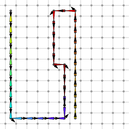
Dual 0-form \(\rho\) is the input of the Poisson problem. Left foot has positive value and right foot has negative value.

Calculus::DualForm0 rho(calculus);
for (int index=0; index<rho.length(); index++)
{
const Calculus::SCell cell = rho.getSCell(index);
const Calculus::Point point = kspace.sKCoords(cell);
if (point[2]>1) continue;
rho.myContainer(index) = point[1]>100 ? 1 : -1;
}
trace.info() << "rho_range=" << rho.myContainer.minCoeff() << "/" << rho.myContainer.maxCoeff() << endl;
const Point & sKCoords(const SCell &c) const
Return its Khalimsky coordinates.
Z3i::SCell SCell
Input dual 0-form.

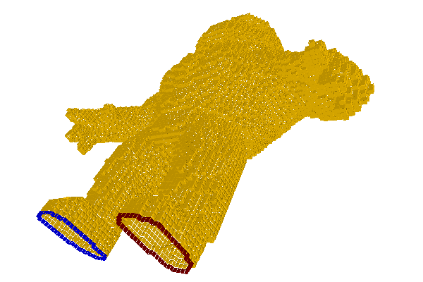
Dual Laplace operator is computed and passed to the solver using DiscreteExteriorCalculusSolver.compute. The dual 0-form solution \(\phi\) is returned by DiscreteExteriorCalculusSolver.solve.

const Calculus::DualIdentity0 laplace = calculus.laplace<DUAL>();
PoissonSolver solver;
solver.compute(laplace);
const Calculus::DualForm0 phi = solver.solve(rho);
trace.info() << "phi_range=" << phi.myContainer.minCoeff() << "/" << phi.myContainer.maxCoeff() << endl;
Aim: This wraps a linear algebra solver around a discrete exterior calculus.
DiscreteExteriorCalculusSolver & compute(const Operator &linear_operator)
Eigen::SparseLU< SparseMatrix > SolverSparseLU
Definition: EigenSupport.h:109
Solution dual 0-form.