Visualization Tools

2dCompImage

Usage: 2dCompImage <imageA>.pgm <imageB>.pgm –imageError <name>Allowed options are :

Positionals:
  1 TEXT:FILE REQUIRED                  Input filename of image A.
  2 TEXT:FILE REQUIRED                  Input filename of image B.
 
Options:
  -h,--help                             Print this help message and exit
  -a,--imageA TEXT:FILE REQUIRED        Input filename of image A.
  -b,--imageB TEXT:FILE REQUIRED        Input filename of image B.
  -e,--imageError TEXT                  Output error image basename (will generate two images <basename>MSE.ppm and <basename>MAE.ppm).
  -S,--setMaxColorValueMSE INT          Set the maximal color value for the scale display of MSE (else the scale is set the maximal MSE value).
  -A,--setMaxColorValueMAE INT          Set the maximal color value for the scale display of MAE (else the scale is set from the maximal MAE value).

Example: Typical use example:

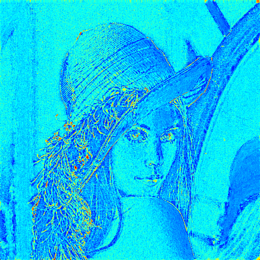
2dCompImage  imageA.pgm imageB.pgm -e errorImage -S 100

You should obtain such a visualisation:

resulting visualisation of absolute error between two images.

See also

2dCompImage.cpp

3DCompSurfelData

Usage: 3dCompSurfelData [input] [reference]Allowed options are:

Positionals:
  1 TEXT:FILE REQUIRED                  input file: sdpa (sequence of discrete points with attribute)
  s TEXT:FILE                           input file: sdpa (sequence of discrete points with attribute)
 
Optionals:
  -h,--help                             Print this help message and exit
  -i,--input TEXT:FILE REQUIRED         input file: sdpa (sequence of discrete points with attribute)
  -r,--reference TEXT:FILE REQUIRED     input file: sdpa (sequence of discrete points with attribute)
  -l,--compAccordingLabels              apply the comparisos only on points with same labels (by default fifth colomn)
  -a,--drawSurfelAssociations           Draw the surfel association.
  -o,--fileMeasureOutput TEXT           specify the output file to store (append) the error stats else the result is given to std output.
  -n,--noWindows                        Don't display Viewer windows.
  -d,--doSnapShotAndExit TEXT           save display snapshot into file. Notes that  the camera setting is set by default according the last saved configuration (use SHIFT+Key_M to save current camera setting in the Viewer3D).
  --fixMaxColorValue FLOAT              fix the maximal color value for the scale error display (else the scale is set from the maximal value)
  --labelIndex UINT                     set the index of the label (by default set to 4)
  --SDPindex UINT x 4                   specify the sdp index (by default 0,1,2,3).

Example: To use this tools we need first to have two differents surfel set with an attribute to be compared. We can use for instance the curvature from the sample file of DGtal/examples/samples/cat10.vol:

# generating another input vol file using tutorial example (eroded.vol):
$ $DGtal/build/examples/tutorial-examples/FMMErosion
# Estimate curvature using other DGtalTools program:
$ 3dCurvatureViewer -i $DGtal/examples/samples/cat10.vol -r 3 --exportOnly -d curvatureCat10R3.dat
$ 3dCurvatureViewer -i eroded.vol -r 3 --exportOnly -d curvatureCat10ErodedR3.dat

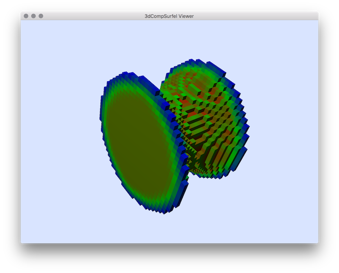
Now we compare the different curvature values from the two shapes:

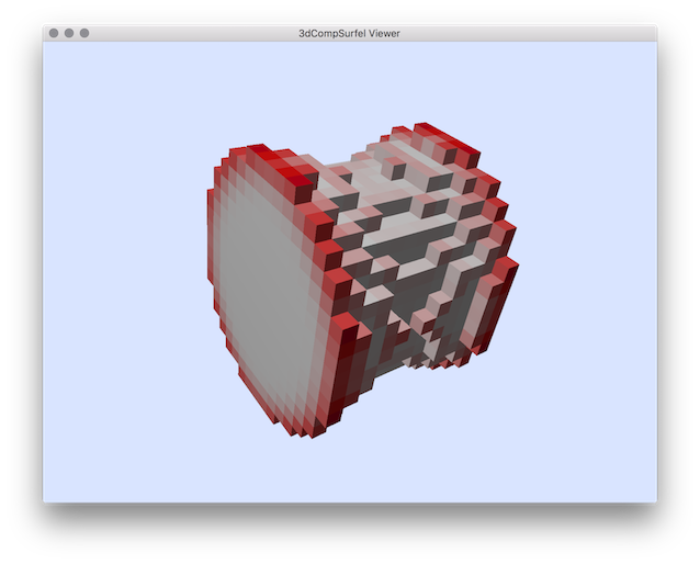
./visualisation/3dCompSurfelData  curvatureCat10ErodedR3.dat curvatureCat10R3.dat --fixMaxColorValue 1.0  -o  statMeasures.dat                       

You should obtain such a visualisation:

resulting visualisation of curvature comparison.

See also

3dCompSurfelData.cpp 3dCurvatureViewer

3DCurvatureViewer

Vol file viewer, with curvature (mean or Gaussian, see parameters) information on surface. Blue color means lowest curvature Yellow color means highest curvature Red means the in-betweenUses IntegralInvariantCurvatureEstimation

See also

related article: Coeurjolly, D.; Lachaud, J.O; Levallois, J., (2013). Integral based Curvature Estimators in Digital Geometry. DGCI 2013. Retrieved from https://liris.cnrs.fr/publis/?id=5866

Usage: 3dCurvatureViewer -i file.vol –radius 5 –mode meanAllowed options are:

Positionals:
  1 TEXT:FILE REQUIRED                  vol file (.vol, .longvol .p3d, .pgm3d and if DGTAL_WITH_ITK is selected: dicom, dcm, mha, mhd). For longvol, dicom, dcm, mha or mhd formats, the input values are linearly scaled between 0 and 255.
 
Options:
  -h,--help                             Print this help message and exit
  -i,--input TEXT:FILE REQUIRED         vol file (.vol, .longvol .p3d, .pgm3d and if DGTAL_WITH_ITK is selected: dicom, dcm, mha, mhd). For longvol, dicom, dcm, mha or mhd formats, the input values are linearly scaled between 0 and 255.
  -r,--radius FLOAT REQUIRED            Kernel radius for IntegralInvariant
  -t,--threshold UINT=8                 Min size of SCell boundary of an object
  -l,--minImageThreshold INT=0          set the minimal image threshold to define the image object (object defined by the voxel with intensity belonging to ]minImageThreshold, maxImageThreshold ] ).
  -u,--maxImageThreshold INT=255        set the maximal image threshold to define the image object (object defined by the voxel with intensity belonging to ]minImageThreshold, maxImageThreshold] ).
  -m,--mode TEXT:{mean,gaussian,k1,k2,prindir1,prindir2,normal}=mean
                                        type of output : mean, gaussian, k1, k2, prindir1, prindir2 or normal(default mean)
  -o,--exportOBJ TEXT                   Export the scene to specified OBJ/MTL filename (extensions added).
  -d,--exportDAT TEXT                   Export resulting curvature (for mean, gaussian, k1 or k2 mode) in a simple data file each line representing a surfel.
  --exportOnly                          Used to only export the result without the 3d Visualisation (usefull for scripts).
  -s,--imageScale FLOAT x 3             scaleX, scaleY, scaleZ: re sample the source image according with a grid of size 1.0/scale (usefull to compute curvature on image defined on anisotropic grid). Set by default to 1.0 for the three axis.
  -n,--normalization BOOLEAN            When exporting to OBJ, performs a normalization so that the geometry fits in [-1/2,1/2]^3

Below are the different available modes:

    - "mean" for the mean curvature
    - "gaussian" for the Gaussian curvature
    - "k1" for the first principal curvature
    - "k2" for the second principal curvature
    - "prindir1" for the first principal curvature direction
    - "prindir2" for the second principal curvature direction
    - "normal" for the normal vector

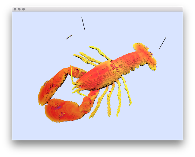
Example: Now we compare the different curvature values from the two shapes:

3dCurvatureViewer  $DGtal/examples/samples/lobster.vol -r 10 -l 40 -u 255 -m mean

You should obtain such a visualisation:

resulting visualisation of mean curvature.

See also

3dCurvatureViewer.cpp, 3DCurvatureViewerNoise

3DCurvatureViewerNoise

Vol file viewer, with curvature (mean or Gaussian, see parameters) information on surface. Blue color means lowest curvature Yellow color means highest curvature Red means the in-betweenUses IntegralInvariantCurvatureEstimation

See also

related article: Coeurjolly, D.; Lachaud, J.O; Levallois, J., (2013). Integral based Curvature Estimators in Digital Geometry. DGCI 2013. Retrieved from https://liris.cnrs.fr/publis/?id=5866

Usage: 3dCurvatureViewerNoise -i file.vol –radius 5 –mode mean –noise 0.5Allowed options are:

Positionals:
  1 TEXT:FILE REQUIRED                  vol file (.vol, .longvol .p3d, .pgm3d and if DGTAL_WITH_ITK is selected: dicom, dcm, mha, mhd). For longvol, dicom, dcm, mha or mhd formats, the input values are linearly scaled between 0 and 255.
 
Options:
  -h,--help                             Print this help message and exit
  -i,--input TEXT:FILE REQUIRED         vol file (.vol, .longvol .p3d, .pgm3d and if DGTAL_WITH_ITK is selected: dicom, dcm, mha, mhd). For longvol, dicom, dcm, mha or mhd formats, the input values are linearly scaled between 0 and 255.
  -r,--radius FLOAT REQUIRED            Kernel radius for IntegralInvariant
  -k,--noise FLOAT=0.5                  Level of Kanungo noise ]0;1[
  -t,--threshold UINT=8                 Min size of SCell boundary of an object
  -l,--minImageThreshold INT=0          set the minimal image threshold to define the image object (object defined by the voxel with intensity belonging to ]minImageThreshold, maxImageThreshold ] ).
  -u,--maxImageThreshold INT=255        set the maximal image threshold to define the image object (object defined by the voxel with intensity belonging to ]minImageThreshold, maxImageThreshold] ).
  -m,--mode TEXT:{mean,gaussian,k1,k2,prindir1,prindir2,normal}=mean
                                        type of output : mean, gaussian, k1, k2, prindir1, prindir2 or normal(default mean)
  -o,--exportOBJ TEXT                   Export the scene to specified OBJ/MTL filename (extensions added).
  -d,--exportDAT TEXT                   Export resulting curvature (for mean, gaussian, k1 or k2 mode) in a simple data file each line representing a surfel.
  --exportOnly                          Used to only export the result without the 3d Visualisation (usefull for scripts).
  -s,--imageScale FLOAT x 3             scaleX, scaleY, scaleZ: re sample the source image according with a grid of size 1.0/scale (usefull to compute curvature on image defined on anisotropic grid). Set by default to 1.0 for the three axis.
  -n,--normalization BOOLEAN            When exporting to OBJ, performs a normalization so that the geometry fits in [-1/2,1/2]^3

Below are the different available modes:

    - "mean" for the mean curvature
    - "gaussian" for the Gaussian curvature
    - "k1" for the first principal curvature
    - "k2" for the second principal curvature
    - "prindir1" for the first principal curvature direction
    - "prindir2" for the second principal curvature direction
    - "normal" for the normal vector

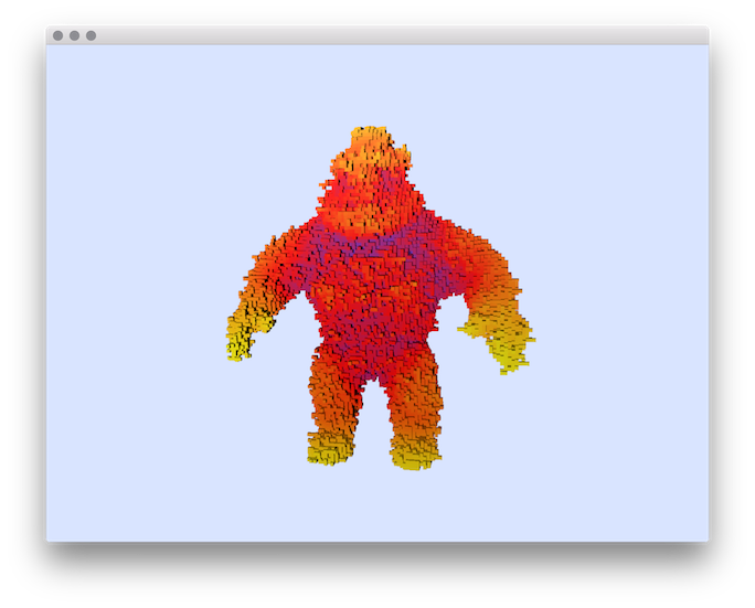
Example:

$ 3dCurvatureViewerNoise $DGtal/examples/samples/Al.100.vol -r 15 -m mean -k 0.5

You should obtain such a visualisation:

resulting visualisation of mean curvature.

See also

3dCurvatureViewerNoise.cpp, 3DCurvatureViewer

3dCurveViewer

Usage: 3dCurveViewer [options] inputAllowed options are :

Positionals:
  1 TEXT:FILE REQUIRED                  the name of the text file containing the list of 3D points (x y z per line).
 
Options:
  -h,--help                             Print this help message and exit
  -i,--input TEXT:FILE REQUIRED         the name of the text file containing the list of 3D points (x y z per line).
  -b,--box INT=0                        specifies the the tightness of the bounding box around the curve with a given integer displacement <arg> to enlarge it (0 is tight)
  -v,--viewBox TEXT:{WIRED,COLORED}=WIRED
                                        displays the bounding box, <arg>=WIRED means that only edges are displayed, <arg>=COLORED adds colors for planes (XY is red, XZ green, YZ, blue).
  -C,--curve3d                          displays the 3D curve.
  -c,--curve2d                          displays the 2D projections of the 3D curve on the bounding box.
  -3,--cover3d                          displays the 3D tangential cover of the curve.
  -2,--cover2d                          displays the 2D projections of the 3D tangential cover of the curve
  -n,--nbColors INT=3                   sets the number of successive colors used for displaying 2d and 3d maximal segments (default is 3: red, green, blue)
  -t,--tangent                          displays the tangents to the curve

Example:

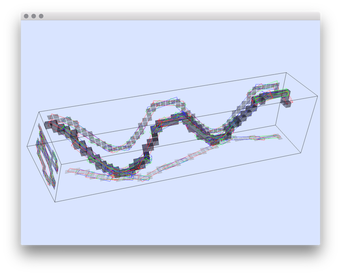
$  3dCurveViewer -C -b 1 -3 -2 -c ${DGtal}/examples/samples/sinus.dat

You should obtain such a visualisation:

resulting visualisation of 3d curve with tangential cover.

See also

3dCurveViewer.cpp

3dDisplaySurfelData

Usage: 3dDisplaySurfelData [OPTIONS] 1 [fixMaxColorValue] [fixMinColorValue]Allowed options are :

Positionals:
  1 TEXT:FILE REQUIRED                  input file: sdp (sequence of discrete points with attribute)
 
Options:
  -h,--help                             Print this help message and exit
  -i,--input TEXT:FILE REQUIRED         input file: sdp (sequence of discrete points with attribute)
  -n,--noWindows                        Don't display Viewer windows.
  -d,--doSnapShotAndExit TEXT           save display snapshot into file.
  --labelIndex UINT                     set the index of the label (by default set to 3)
  --SDPindex UINT ...                   specify the sdp index (by default 0,1,2).
  --fixMaxColorValue FLOAT              fix manually the maximal color value for the scale error display (else the scale is set from the maximal value)
 --fixMinColorValue FLOAT               fix manually the maximal color value for the scale error display (else the scale is set from the minimal value)

Example: To test this program we have first to generate a file containing a set of surfels with, for instance, their associated curvature values:

$ 3dCurvatureViewer -i $DGtal/examples/samples/cat10.vol -r 3 --exportOnly -d curvatureCat10R3.dat

Then, we can use this tool to display the set of surfel with their associated values:

$ 3dDisplaySurfelData -i curvatureCat10R3.dat 

You should obtain such a result:

resulting visualisation of surfel with their associated values.

See also

3dDisplaySurfelData.cpp, 3DCompSurfelData

3dHeightMapViewer

Usage: 3dImageViewer [options] inputAllowed options are :

Positionals:
  1 TEXT:FILE REQUIRED                  2d input image representing the height map (given as grayscape image cast into 8 bits).
 
Options:
  -h,--help                             Print this help message and exit
  -i,--input TEXT:FILE REQUIRED         2d input image representing the height map (given as grayscape image cast into 8 bits).
  -s,--scale FLOAT                      set the scale of the maximal level. (default 1.0)
  -c,--colorMap                         define the heightmap color with a pre-defined colormap (GradientColorMap)
  -t,--colorTextureImage TEXT           define the heightmap color from a given color image (32 bits image).

Example:

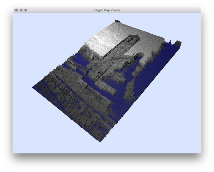
$ visualisation/3dHeightMapViewer ${DGtal}/examples/samples/church.pgm -s 0.2

You should obtain such a result:

resulting heightmap visualisation.

See also

3dHeightMapViewer.cpp

3dImageViewer

Usage: 3dImageViewer [OPTIONS] 1 [s]Allowed options are :

Positionals:
  1 TEXT:FILE REQUIRED                  vol file (.vol, .longvol .p3d, .pgm3d and if DGTAL_WITH_ITK is selected: dicom, dcm, mha, mhd). For longvol, dicom, dcm, mha or mhd formats, the input values are linearly scaled between 0 and 255.
  s TEXT                                display a set of discrete points (.sdp)
 
Options:
  -h,--help                             Print this help message and exit
  -i,--input TEXT:FILE REQUIRED         vol file (.vol, .longvol .p3d, .pgm3d and if DGTAL_WITH_ITK is selected: dicom, dcm, mha, mhd). For longvol, dicom, dcm, mha or mhd formats, the input values are linearly scaled between 0 and 255.
  --grid                                draw slice images using grid mode.
  --intergrid                           draw slice images using inter grid mode.
  --emptyMode                           remove the default boundingbox display.
  --thresholdImage                      threshold the image to define binary shape
  --thresholdMin INT=0                  threshold min to define binary shape
  --thresholdMax INT=255                threshold maw to define binary shape
  --displaySDP TEXT                     display a set of discrete points (.sdp)
  --SDPindex UINT x 3                   specify the sdp index.
  --SDPball FLOAT=0                     use balls to display a set of discrete points (if not set to 0 and used with displaySDP option).
  --displayMesh TEXT                    display a Mesh given in OFF or OFS format.
  --displayDigitalSurface               display the digital surface instead of display all the set of voxels (used with thresholdImage or displaySDP options)
  --colorizeCC                          colorize each Connected Components of the surface displayed by displayDigitalSurface option.
  -c,--colorSDP UINT x 4                set the color  discrete points: r g b a
  --colorMesh UINT x 4                  set the color of Mesh (given from displayMesh option) : r g b a
  -x,--scaleX FLOAT=1                   set the scale value in the X direction
  -y,--scaleY FLOAT=1                   set the scale value in the Y direction
  -z,--scaleZ FLOAT=1                   set the scale value in the Z direction
  --rescaleInputMin INT=0               min value used to rescale the input intensity (to avoid basic cast into 8  bits image).
  --rescaleInputMax INT=255             max value used to rescale the input intensity (to avoid basic cast into 8  bits image).
  -t,--transparency UINT=?              change the default transparency

Example: With the image display you can also threshold the image and display a set of voxel:

3dImageViewer $DGtal/examples/samples/lobster.vol --thresholdImage -m 180

You should obtain such a result:

resulting visualisation of 3d image with thresholded set of voxels.

See also

3dImageViewer.cpp

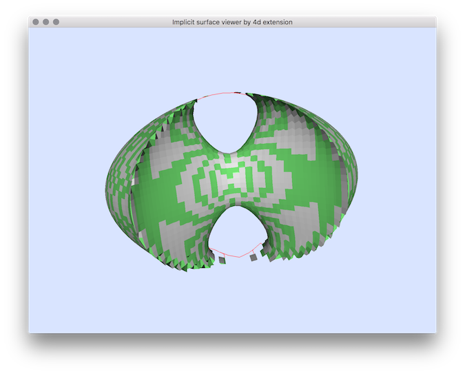
3dImplicitSurfaceExtractorBy4DExtension

Usage: 3dImplicitSurfaceExtractorBy4DExtension [options] inputAllowed options are :

-h [ --help ]                         display this message
-p [ --polynomial ] arg               the implicit polynomial whose 
                                      zero-level defines the shape of 
                                      interest.
-a [ --minAABB ] arg (=-10)           the min value of the AABB bounding box 
                                      (domain)
-A [ --maxAABB ] arg (=10)            the max value of the AABB bounding box 
                                      (domain)
-g [ --gridstep ] arg (=1)            the gridstep that defines the 
                                      digitization (often called h). 
-t [ --timestep ] arg (=9.9999999999999995e-07)
                                      the gridstep that defines the 
                                      digitization in the 4th dimension 
                                      (small is generally a good idea, 
                                      default is 1e-6). 
-P [ --project ] arg (=Newton)        defines the projection: either No or 
                                      Newton.
-e [ --epsilon ] arg (=9.9999999999999995e-08)
                                      the maximum precision relative to the 
                                      implicit surface.
-n [ --max_iter ] arg (=500)          the maximum number of iteration in the 
                                      Newton approximation of F=0.
-v [ --view ] arg (=Normal)           specifies if the surface is viewed as 
                                      is (Normal) or if places close to 
                                      singularities are highlighted 
                                      (Singular).

Example:

3dImplicitSurfaceExtractorBy4DExtension -p "-0.9*(y^2+z^2-1)^2-(x^2+y^2-1)^3" -g 0.06125 -a -2 -A 2 -v Singular -t 0.02

You could also use other implicit surfaces:

• whitney : x^2-y*z^2
• 4lines : x*y*(y-x)*(y-z*x)
• cone : z^2-x^2-y^2
• simonU : x^2-z*y^2+x^4+y^4
• cayley3 : 4*(x^2 + y^2 + z^2) + 16*x*y*z - 1
• crixxi : -0.9*(y^2+z^2-1)^2-(x^2+y^2-1)^3

You should obtain such a result:

resulting visualisation.

See also

3dImplicitSurfaceExtractorBy4DExtension.cpp

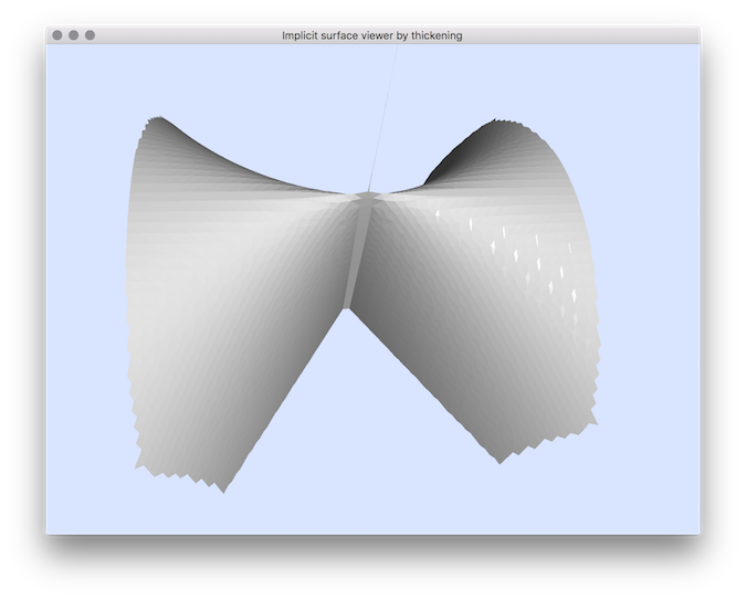
3dImplicitSurfaceExtractorByThickening

Usage: 3dImplicitSurfaceExtractorByThickening [options] inputAllowed options are :

ositionals:
  1 TEXT REQUIRED                       the implicit polynomial whose zero-level defines the shape of interest.
 
Options:
  -h,--help                             Print this help message and exit
  -p,--polynomial TEXT REQUIRED         the implicit polynomial whose zero-level defines the shape of interest.
  -a,--minAABB FLOAT=-10                the min value of the AABB bounding box (domain)
  -A,--maxAABB FLOAT=10                 the max value of the AABB bounding box (domain)
  -g,--gridstep FLOAT=1                 the gridstep that defines the digitization (often called h).
  -t,--thickness FLOAT=0.01             the thickening parameter for the implicit surface.
  -P,--project TEXT:{No,Newton}=Newton  defines the projection: either No or Newton.
  -e,--epsilon FLOAT=1e-06              the maximum precision relative to the implicit surface in the Newton approximation of F=0.
  -n,--max_iter UINT=500                the maximum number of iteration in the Newton approximation of F=0.
  -o,--obj TEXT                         OBJ export filename.
  -v,--view TEXT:{Singular,Normal,Hide}=Normal
                                        specifies if the surface is viewed as is (Normal) or if places close to singularities are highlighted (Singular), or if unsure places should not be displayed (Hide).

Example:

3dImplicitSurfaceExtractorByThickening "x^2-y*z^2" -g 0.1 -a -2 -A 2 -v Singular

You should obtain such a result:

resulting visualisation.

You could also use other implicit surfaces:

• whitney : x^2-y*z^2
• 4lines : x*y*(y-x)*(y-z*x)
• cone : z^2-x^2-y^2
• simonU : x^2-z*y^2+x^4+y^4
• cayley3 : 4*(x^2 + y^2 + z^2) + 16*x*y*z - 1
• crixxi : -0.9*(y^2+z^2-1)^2-(x^2+y^2-1)^3

Some other examples (more difficult):

3dImplicitSurfaceExtractorByThickening -a -2 -A 2  "((y^2+z^2-1)^2-(x^2+y^2-1)^3)*(y*(x-1)^2-z*(x+1))^2" -g 0.025 -e 1e-6 -n 50000 -v Singular -t 0.5 -P Newton
3dImplicitSurfaceExtractorByThickening -a -2 -A 2  "(x^5-4*z^3*y^2)*((x+y)^2-(z-x)^3)" -g 0.025 -e 1e-6 -n 50000 -v Singular -t 0.05 -P Newton

See also

3dImplicitSurfaceExtractorByThickening.cpp

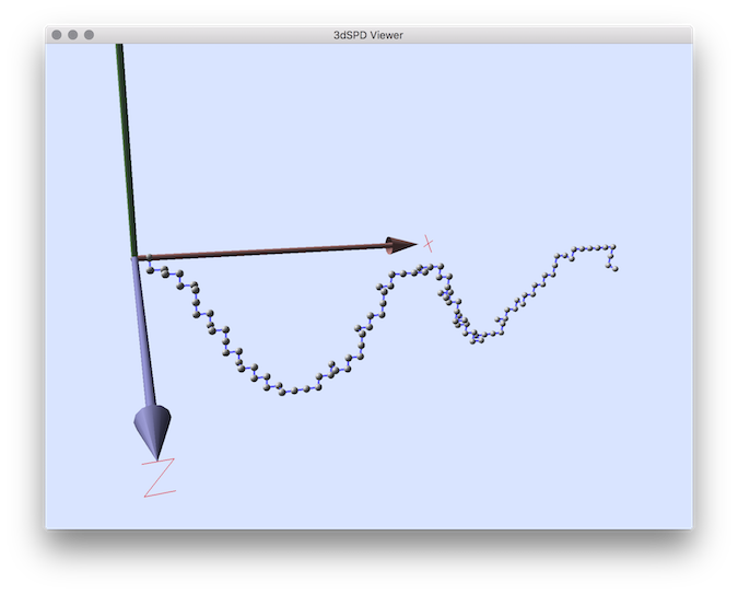
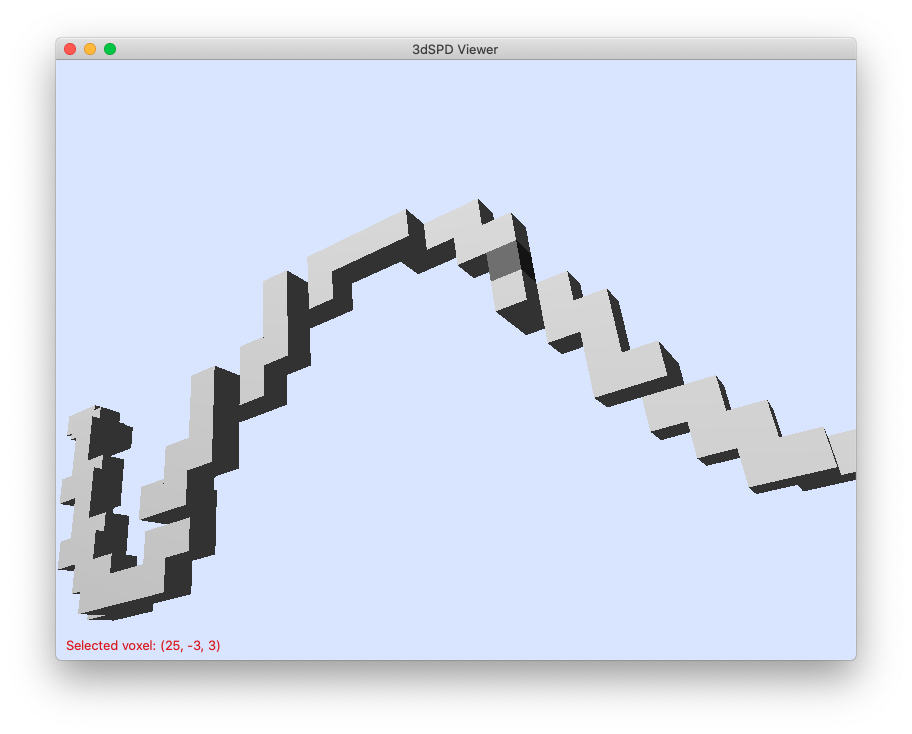
3DSDPViewer

Usage: 3dSDPViewer [OPTIONS] 1 [f] [lineSize] [filterVectors]Allowed options are :

Positionals:
  1 TEXT:FILE REQUIRED                  input file: sdp (sequence of discrete points).
 
Options:
  -h,--help                             Print this help message and exit
  -i,--input TEXT:FILE REQUIRED         input file: sdp (sequence of discrete points).
  --SDPindex UINT x 3                   specify the sdp index (by default 0,1,2).
  -c,--pointColor INT x 4               set the color of  points: r g b a.
  -l,--lineColor INT x 4                set the color of line: r g b a.
  -m,--addMesh TEXT                     append a mesh (off/obj) to the point set visualization.
  --customColorMesh UINT x 4            set the R, G, B, A components of the colors of the mesh faces (mesh added with option --addMesh).
  --customAlphaMesh UINT                set single alpha(A) components of the colors of the mesh faces (mesh added with option --addMesh).
  --importColors                        import point colors from the input file (R G B colors should be by default at index 3, 4, 5).
  --setColorsIndex UINT x 3 Needs: --importColors
                                        customize the index of the imported colors in the source file (used by --importColor). By default the initial indexes are 3, 4, 5.
  --importColorLabels                   import color labels from the input file (label index  should be by default at index 3).
  --setColorLabelIndex UINT=3           customize the index of the imported color labels in the source file (used by -importColorLabels).
  -f,--filter FLOAT=100                 filter input file in order to display only the [arg] percent of the input 3D points (uniformly selected).
  --noPointDisplay                      usefull for instance to only display the lines between points.
  --drawLines                           draw the line between discrete points.
  -x,--scaleX FLOAT=1                   set the scale value in the X direction
  -y,--scaleY FLOAT=1                   set the scale value in the Y direction
  -z,--scaleZ FLOAT=1                   set the scale value in the Z direction
  --sphereResolution UINT=30            defines the sphere resolution (used when the primitive is set to the sphere).
  -s,--sphereRadius FLOAT=0.2           defines the sphere radius (used when the primitive is set to the sphere).
  --sphereRadiusFromInput               takes, as sphere radius, the 4th field of the sdp input file.
  --lineSize FLOAT=0.2                  defines the line size (used when the --drawLines or --drawVectors option is selected).
  -p,--primitive TEXT:{voxel,glPoints,sphere}=voxel
                                        set the primitive to display the set of points.
  -v,--drawVectors TEXT                 SDP vector file: draw a set of vectors from the given file (each vector are determined by two consecutive point given, each point represented by its coordinates on a single line.
  -u,--unitVector FLOAT=0               specifies that the SDP vector file format (of --drawVectors option) should be interpreted as unit vectors (each vector position is be defined from the input point (with input order) with a constant norm defined by [arg]).
  --filterVectors FLOAT=100             filters vector input file in order to display only the [arg] percent of the input vectors (uniformly selected, to be used with option --drawVectors else no effect).
  --interactiveDisplayVoxCoords          by using this option the coordinates can be displayed after selection (shift+left click on voxel).

Basic example: You can display a set of 3D points with sphere primitive and lines:

$  3DSDPViewer  $DGtal/tests/samples/sinus3D.dat -p sphere -s 0.3 --drawLines --lineSize 5

You should obtain such a result:

Resulting visualization.

Example with interactive selection :This tool can be useful to recover coordinates from a set of voxels. To do it, you have to add the option allowing to activate the interactive selection (with –interactiveDisplayVoxCoords), for instance if you apply:

$ 3dSDPViewer  $DGtal/tests/samples/sinus3D.dat  --interactiveDisplayVoxCoords

you should be able to select a voxel by using the SHIFT key and by clicking on a voxel:

Visualization of large point set If you need to display an important number of points, you can use the primitive glPoints instead voxel or sphere (-p glPoints). You will obtain such type of a visualization:

See also

3DSDPViewer.cpp

3dVolBoundaryViewer

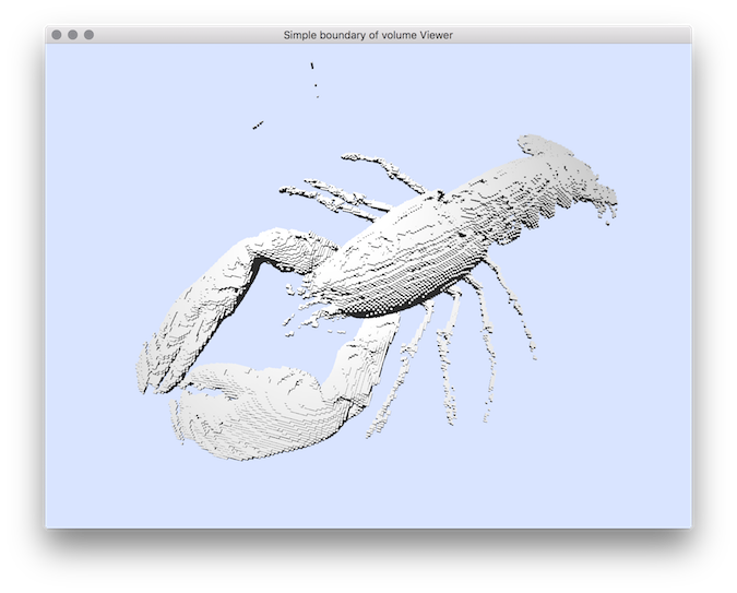
The mode specifies if you wish to see surface elements (BDRY), the inner voxels (INNER) or the outer voxels (OUTER) that touch the boundary.Usage: 3dVolBoundaryViewer -i [input]Allowed options are :

Positionals:
1 TEXT:FILE REQUIRED                  vol file (.vol, .longvol .p3d, .pgm3d and if DGTAL_WITH_ITK is selected: dicom, dcm, mha, mhd). For longvol, dicom, dcm, mha or mhd formats, the input values are linearly scaled between 0 and 255.
 
Options:
-h,--help                             Print this help message and exit
-i,--input TEXT:FILE REQUIRED         vol file (.vol, .longvol .p3d, .pgm3d and if DGTAL_WITH_ITK is selected: dicom, dcm, mha, mhd). For longvol, dicom, dcm, mha or mhd formats, the input values are linearly scaled between 0 and 255.
-m,--thresholdMin INT=0               threshold min (excluded) to define binary shape.
-M,--thresholdMax INT=255             threshold max (included) to define binary shape.
--mode TEXT:{INNER,OUTER,BDRY}=INNER  set mode for display: INNER: inner voxels, OUTER: outer voxels, BDRY: surfels
OUTER: outer voxels, BDRY: surfels

Example:

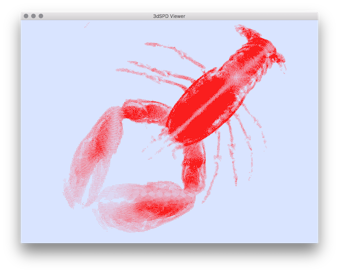
3dVolBoundaryViewer  $DGtal/examples/samples/lobster.vol -m 60

You should obtain such a result:

Resulting visualization.

See also

3dVolBoundaryViewer.cpp

3dVolViewer

The mode specifies if you wish to see surface elements (BDRY), the inner voxels (INNER) or the outer voxels (OUTER) that touch the boundary.Usage: 3dVolViewer [input]Allowed options are :

Positionals:
  1 TEXT:FILE REQUIRED                  vol file (.vol, .longvol .p3d, .pgm3d and if DGTAL_WITH_ITK is selected: dicom, dcm, mha, mhd). For longvol, dicom, dcm, mha or mhd formats, the input values are linearly scaled between 0 and 255.
 
Options:
  -h,--help                             Print this help message and exit
  -i,--input TEXT:FILE REQUIRED         vol file (.vol, .longvol .p3d, .pgm3d and if DGTAL_WITH_ITK is selected: dicom, dcm, mha, mhd). For longvol, dicom, dcm, mha or mhd formats, the input values are linearly scaled between 0 and 255.
  -m,--thresholdMin INT=0               threshold min (excluded) to define binary shape.
  -M,--thresholdMax INT=255             threshold max (included) to define binary shape.
  --rescaleInputMin INT=0               min value used to rescale the input intensity (to avoid basic cast into 8  bits image).
  --rescaleInputMax INT=255             max value used to rescale the input intensity (to avoid basic cast into 8  bits image).
  -n,--numMaxVoxel UINT                 set the maximal voxel number to be displayed.
  --displayMesh TEXT                    display a Mesh given in OFF or OFS format.
  --colorMesh UINT ...                  set the color of Mesh (given from displayMesh option) : r g b a
  -d,--doSnapShotAndExit                save display snapshot into file. Notes that the camera setting is set by default according the last saved configuration (use SHIFT+Key_M to save current camera setting in the Viewer3D). If the camera setting was not saved it will use the default camera setting.
  -t,--transparency UINT=255            change the defaukt transparency

Example:

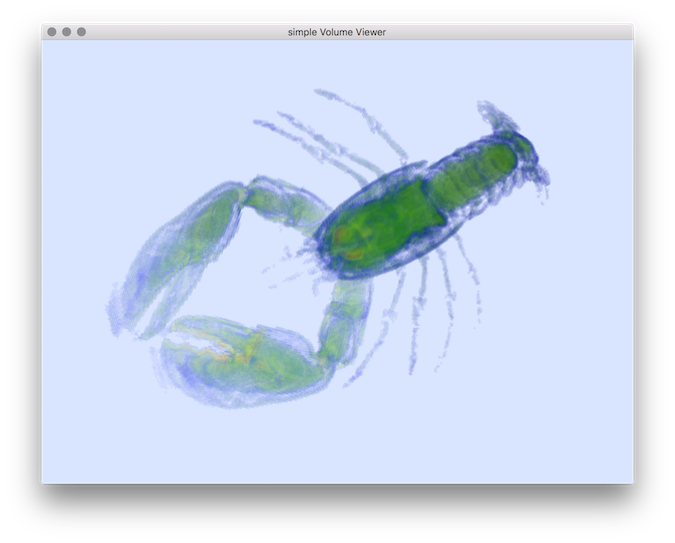
$ 3dVolViewer $DGtal/examples/samples/lobster.vol -m 60 -t 10

You should obtain such a result:

Resulting visualization.

See also

3dVolViewer.cpp

displayContours

Usage: displayContours [options] -i <fileName>Allowed options are :

Positionals:
  1 TEXT:FILE REQUIRED                 input FreemanChain file name
 
Options:
  -h,--help                             Print this help message and exit
  -i,--input TEXT:FILE                  input FreemanChain file name
  -o,--outputFile TEXT                  save output file automatically according the file format extension.
  --SDP TEXT:FILE                       Import a contour as a Sequence of Discrete Points (SDP format)
  --SFP TEXT:FILE                       mport a contour as a Sequence of Floating Points (SFP format)
  --drawContourPoint FLOAT              <size> display contour points as disk of radius <size>
  --fillContour                         fill the contours with default color (gray)
  --lineWidth FLOAT                     Define the linewidth of the contour (SDP format)
  -f,--drawPointOfIndex UINT             Draw the contour point of index.
  --pointSize FLOAT                     <size> Set the display point size of the point displayed by drawPointofIndex option (default 2.0)
  --noXFIGHeader BOOLEAN                to exclude xfig header in the resulting output stream (no effect with option -outputFile).
  --withProcessing TEXT:{MS,FP,MLP}     Processing (used only when the input is a Freeman chain (--input)):
                                           DSS segmentation {DSS}
                                            Maximal segments {MS}
                                           Faithful Polygon {FP}
                                           Minimum Length Polygon {MLP}
  -v,--displayVectorField TEXT          Add the display of a vector field represented by two floating coordinates. Each vector is displayed starting from the corresponding contour point coordinates.
  --scaleVectorField FLOAT=1            set the scale of the vector field (default 1) (used with --displayVectorField).
  --vectorFieldIndex UINT=[0,1] x 2     specify the vector field index (by default 0,1) (used with --displayVectorField).
  --vectorFromAngle UINT                specify that the vectors are defined from an angle value represented at the given index  (by default 0) (used with --displayVectorField).
  --rotateVectorField                   apply a CCW rotation of 90° (used with --displayVectorField).
  --outputStreamEPS                      specify eps for output stream format.
  --outputStreamSVG                      specify svg for output stream format.
  --outputStreamFIG                      specify fig for output stream format.
  --invertYaxis Needs: --SDP             invertYaxis invert the Y axis for display contours (used only with --SDP)
  --backgroundImage TEXT:FILE           backgroundImage <filename> : display image as background
  --alphaBG FLOAT=1                     alphaBG <value> 0-1.0 to display the background image in transparency (default 1.0), (transparency works only if cairo is available)
  --scale FLOAT=1                       scale <value> 1: normal; >1 : larger ; <1 lower resolutions)

Example: In this example we show how to display of a set of contours extracted in a single image. The first step is to extract a set contours by using the tool

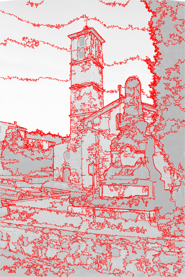
$ img2freeman $DGtal/examples/samples/church.pgm  -R 0 20 255 -s 200  > church.fc

Then, we display the set of contours with the background images (you need to have compiled DGTal with the options (-DWITH_MAGICK=true and -DDGTAL_WITH_CAIRO=true) :

$  displayContours church.fc   --backgroundImage $DGtal/examples/samples/church.png --alphaBG 0.75 --outputFile church.pdf

You should obtain such a result:

Resulting visualization.

See also

displayContours.cpp

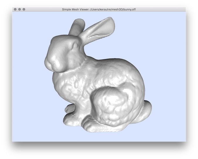
meshViewer

Usage: meshViewer [input]Allowed options are :

Positionals:
1 TEXT:FILE ... REQUIRED              inputFileNames.off files (.off), or OFS file (.ofs)
 
Options:
-h,--help                             Print this help message and exit
-i,--input TEXT:FILE ... REQUIRED     inputFileNames.off files (.off), or OFS file (.ofs)
-x,--scaleX FLOAT                     set the scale value in the X direction (default 1.0)
-y,--scaleY FLOAT                     set the scale value in the y direction (default 1.0)
-z,--scaleZ FLOAT                     set the scale value in the z direction (default 1.0)
--minLineWidth FLOAT=1.5              set the min line width of the mesh faces (default 1.5)
--customColorMesh UINT ...            set the R, G, B, A components of the colors of the mesh faces and eventually the color R, G, B, A of the mesh edge lines (set by default to black).
--customAlphaMesh UINT ...            set the alpha components of the colors of the mesh faces (can be applied for each mesh).
--customColorSDP UINT x 4             set the R, G, B, A components of the colors of  the sdp view
-f,--displayVectorField TEXT          display a vector field from a simple sdp file (two points per line)
--vectorFieldIndex UINT x 6           specify special indices for the two point coordinates (instead usinf the default indices: 0 1, 2, 3, 4, 5)
--customLineColor UINT x 4            set the R, G, B components of the colors of the lines displayed from the --displayVectorField option (red by default).
--SDPradius FLOAT=0.5                 change the ball radius to display a set of discrete points (used with displaySDP option)
-s,--displaySDP TEXT                  add the display of a set of discrete points as ball of radius 0.5.
-A,--addAmbientLight FLOAT            add an ambient light for better display (between 0 and 1).
-b,--customBGColor UINT x 3           set the R, G, B components of the colors of the background color.
-d,--doSnapShotAndExit TEXT           save display snapshot into file. Notes that the camera                                             setting is set by default according the last saved                                                 configuration (use SHIFT+Key_M to save current camera                                              setting in the Viewer3D). If the camera setting was not                                            saved it will use the default camera setting.
-l,--fixLightToScene                  Fix light source to scence instead to camera
-n,--invertNormal                     invert face normal vectors.
-v,--drawVertex                       draw the vertex of the mesh

Example:

$ meshViewer bunny.off

You should obtain such a result:

Resulting visualization.

See also

meshViewer.cpp

patternTriangulation

Usage: patternTriangulation -a 5 -b 8Allowed options are :

Options:
  -h,--help                             Print this help message and exit
  -a,--aparam INT REQUIRED              pattern a parameter
  -b,--bparam INT REQUIRED              pattern b parameter
  -d,--delta INT                        number of repetitions
  -t,--triangulation TEXT=CH            output:
                                                Closest-point Delaunay triangulation {CDT}
                                                Farthest-point Delaunay triangulation {FDT}
                                                Convex hull {CH}

Example:

$ patternTriangulation -a 5 -b 8 

Result: a=5, b=8, d=1

See also

patternTriangulation.cpp

volscope

Usage: volscope [options] –input <fileName>Allowed options are :

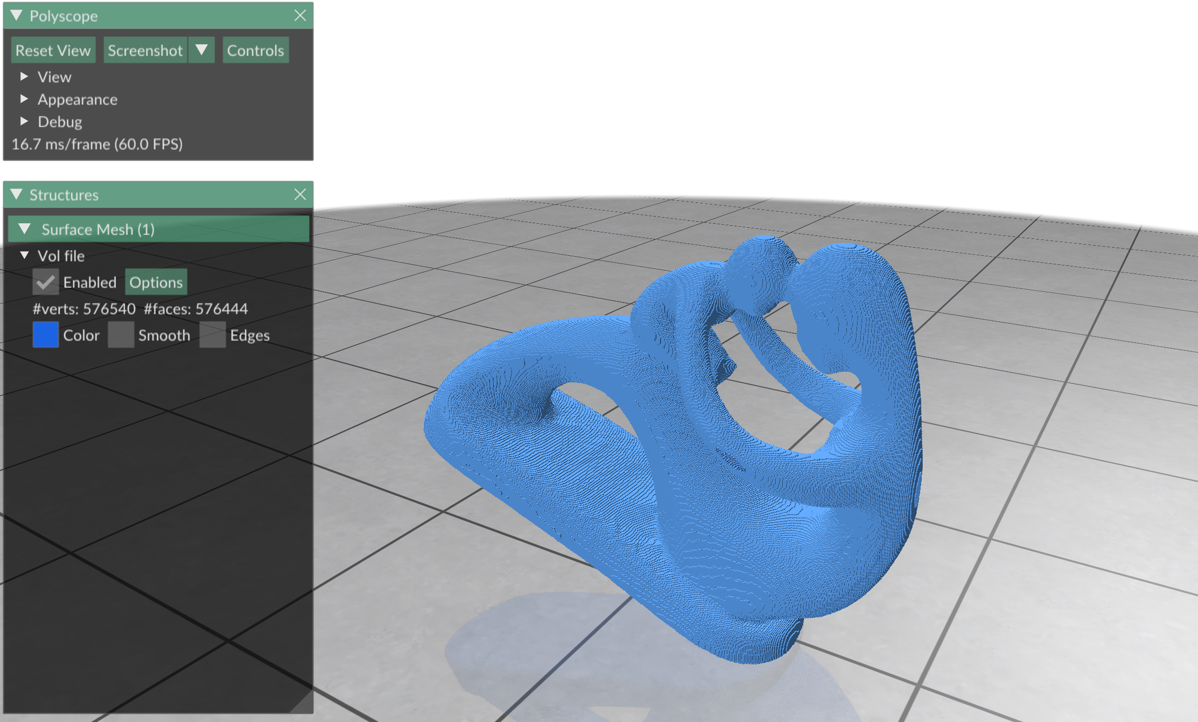
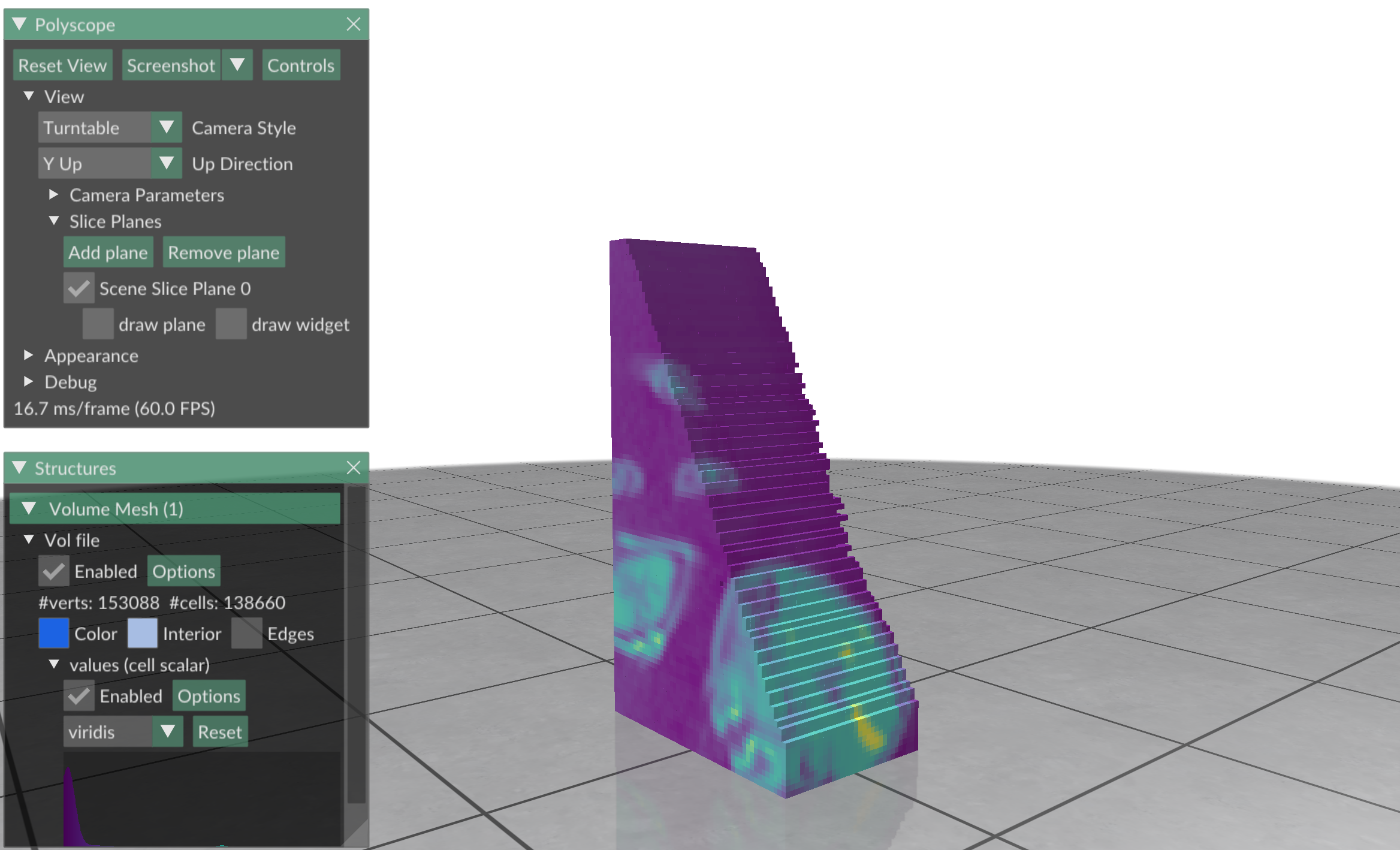
 Usage: ./volscope [OPTIONS] 1
 
 Positionals:
 1 TEXT:FILE REQUIRED                  Input vol file.
 
 Options:
 -h,--help                             Print this help message and exit
 -i,--input TEXT:FILE REQUIRED         Input vol file.
 --volumetricMode                      Activate the volumetric mode instead of the isosurface visualization.
 --point-cloud-only                    In the volumetric mode, visualize the vol file as a point cloud instead of an hex mesh (default: false)
-m,  --min INT                             For isosurface visualization and voxel filtering, specifies the threshold min (excluded) (default: 0).
 -M, --max INT                             For isosurface visualization and voxel filtering, specifies the threshold max (included) (default: 255).

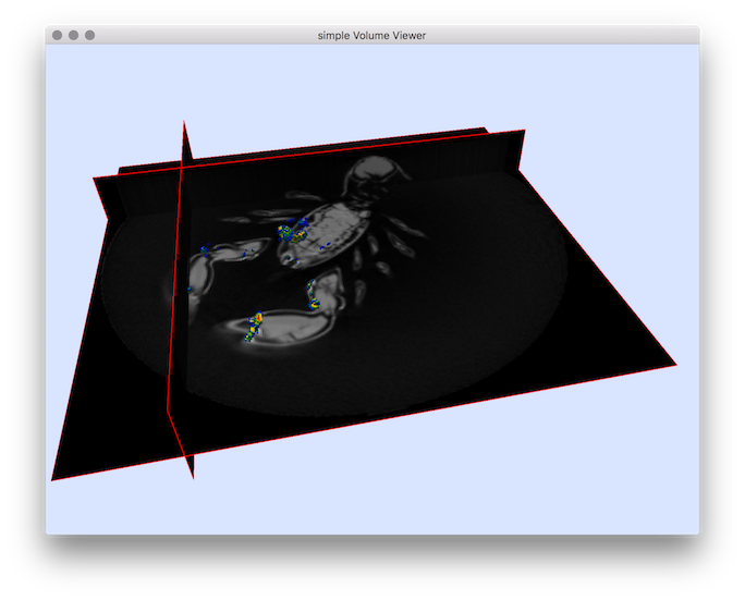
Default visualization mode.

Volumetric visualization using polyscope slice planes.