Table of Contents
- Author(s) of this documentation:
- Jacques-Olivier Lachaud
- Since
- 1.1
Part of the Geometry package.
This part of the manual describes tools associated to a new definition of digital convexity, called the full convexity [80] [81] . This new definition solves many problems related to the usual definition of digital convexity, like possible non connectedness or non simple connectedness, while encompassing its desirable features. Fully convex sets are digitally convex, but are also connected and simply connected. They have a morphological characterisation, which induces a simple convexity test algorithm. As an important example, arithmetic planes are fully convex too. Since DGtal release 1.5, P-convexity can also be checked in arbitrary dimension. It is worth to note that it is equivalent to full convexity, and is generally faster to check [55] .
The following programs are related to this documentation: geometry/curves/exampleDigitalConvexity.cpp, geometry/curves/exampleRationalConvexity.cpp, testBoundedLatticePolytope.cpp, testBoundedLatticePolytopeCounter.cpp, testCellGeometry.cpp, testDigitalConvexity.cpp, testEhrhartPolynomial.cpp, geometry/volumes/exampleBoundedLatticePolytopeCount2D.cpp, geometry/volumes/exampleBoundedLatticePolytopeCount3D.cpp, geometry/volumes/exampleBoundedLatticePolytopeCount4D.cpp, geometry/volumes/pConvexity-benchmark.cpp .
This module relies on module QuickHull algorithm in arbitrary dimension for convex hull and Delaunay cell complex computation for convex hull computations in arbitrary dimensions.
You may also look at Applications of full digital convexity to see some applications of full convexity.
See Fully convex envelope, relative fully convex envelope and digital polyhedra to see how to build fully convex hulls and digital polyhedra.
Introduction to full convexity
The usual definition for digital convexity is as follows. For some digital set \( S \subset \mathbb{Z}^d \), \( S \) is said to be digitally convex whenever \( \mathrm{Conv}(S) \cap \mathbb{Z}^d = S \). Otherwise said, the convex hull of all the digital points contains exactly these digital points and no other.
Although handy and easy to check, this definition lacks many properties related to (continuous) convexity in the Euclidean plane.
We extend this definition as follows (see [80] [81] ). Let \( C^d \) be the usual regular cubical complex induced by the lattice \( \mathbb{Z}^d \), and let \( C^d_k \) be its k-cells, for \( 0 \le k \le d \). We have that the 0-cells of \( C^d_0 \) are exactly the lattice points, the 1-cells of \( C^d_1 \) are the open unit segment joining 2 neighboring lattice points, etc.
Finally, for an arbitrary subset \( Y \subset \mathbb{R}^d \), we denote by \( C^d_k \lbrack Y \rbrack \) the set of k-cells of \( C^d \) whose closure have a non-empty intersection with \( Y \), i.e. \( C^d_k \lbrack Y \rbrack := \{ c \in C^d_k,~\text{s.t.}~ \bar{c} \cap Y \neq \emptyset \} \).
A digital set \( S \subset \mathbb{Z}^d \) is said to be digitally k- convex whenever \( C^d_k \lbrack \mathrm{Conv}(S) \rbrack = C^d_k \lbrack S \rbrack \). \( S \) is said to be fully (digitally) convex whenever it is digitally k- convex for \( 0 \le k \le d \).
A fully convex set is always \( 3^d-1 \)-connected (i.e. 8-connected in 2D, 26-connected in 3D). Furthermore its axis-aligned slices are connected (with the same kind of connectedness). It is also clear that digitally 0-convexity is the usual digital convexity.
A last useful notion is the subconvexity, or tangency. Let \( X \subset \mathbb{Z}^d \) some arbitrary digital set. Then the digital set \( S \subset \mathbb{Z}^d \) is said to be digitally k- subconvex to \( X \) whenever \( C^d_k \lbrack \mathrm{Conv}(S) \rbrack \subset C^d_k \lbrack X \rbrack \). And \( S \) is said to be fully (digitally) subconvex to \( X \) whenever it is digitally k- subconvex to \( X \) for \( 0 \le k \le d \).
Subconvexity is a useful for notion for digital contour and surface analysis. It tells which subsets of these digital sets are tangent to them.
The notion of P-convexity has been proposed in [55] . A set \( S \subset \mathbb{Z}^d \) is P-convex if and only if
- \( S \) is 0-convex,
- and, if \( d > 1 \), the $d$ projections of $S$ along each axis is P-convex (in \( \mathbb{Z}^{d-1} \)).
P-convexity is equivalent to full convexity as shown in [55] .
Classes and functions related to digital convexity
Three classes help to check digital convexity.
- BoundedLatticePolytope is the class that is used to build polytopes, i.e. intersections of half-spaces, which are a way to represent convex polyhedra.
- CellGeometry is used to store sets of cells and provides methods to build the set of cells that intersect a polytope or the set of cells that touch a set of digital points.
- DigitalConvexity provides many helper methods to build BoundedLatticePolytope and CellGeometry objects and to check digital convexity and subconvexity.
- PConvexity provides functions to check digital convexity and P-convexity, as well a full convexity measure that is characteristics of full convex sets (or equivalently P-convex sets).
Lattice polytopes
Construction. You have different ways to build the lattice polytope:
- from a full dimensional simplex: you may build a polytope in dimension \( d \le 3 \) from a range of \( n \le d + 1 \) points in general position. The polytope is then a simplex. For dimensions higher than 3, you may only build the polytope from a full dimensional simplex, i.e. \( n = d + 1 \) in general position.
- from a domain and a range of half-spaces: they define obviously a bounded H-polytope.
- from an arbitrary set of points (full dimensional is the dimension is greater or equal to 4) using DigitalConvexity::makePolytope or ConvexityHelper::computeLatticePolytope.
other operations. You may also cut a polytope by a new halfspace (BoundedLatticePolytope::cut), count the number of lattice points inside, interior or on the boundary (BoundedLatticePolytope::count, BoundedLatticePolytope::countInterior, BoundedLatticePolytope::countBoundary) or enumerate them.
- Note
- In versions before 1.3, lattice point counting was done in a naive way, by domain enumeration and constraints check. If m is the number of constraints and n the number of lattice points in the polytope domain, then complexity was in \( O(mn) \).
- Since 1.3, inside/interior point counting and retrieval have been considerably optimized and are between 5x to 200x faster. The code uses line intersection to compute the inside points as intervals. See examples exampleBoundedLatticePolytopeCount2D.cpp , exampleBoundedLatticePolytopeCount3D.cpp , exampleBoundedLatticePolytopeCount4D.cpp .
Last, you may compute Minkowski sums of a polytope with axis-aligned segments, squares or (hyper)-cubes (BoundedLatticePolytope::operator+=).
- Note
- You can check if the result of a Minkowski sum will be valid by calling BoundedLatticePolytope::canBeSummed before. The support is for now limited to polytopes built as simplices in 2D and 3D.
Point check services:
- BoundedLatticePolytope::isInside checks if some point belongs to the polytope.
- BoundedLatticePolytope::isDomainPointInside checks if some point within the polytope bounding box belongs to the polytope.
- BoundedLatticePolytope::isInterior checks if some point is strictly inside the polytope.
- BoundedLatticePolytope::isBoundary checks if some point is lying on the polytope boundary.
Standard polytope services:
- BoundedLatticePolytope::interiorPolytope returns the corresponding interior polytope by making strict every constraint
- BoundedLatticePolytope::cut cuts the polytope by the given half-space constraint
- BoundedLatticePolytope::swap swaps this polytope with another one in constant time
- BoundedLatticePolytope::operator*= dilates this polytope by a given factor
- BoundedLatticePolytope::operator+= performs Minkowski sum with some axis aligned unit segment/cell
Enumeration services:
- BoundedLatticePolytope::count counts the number of lattice points in the polytope
- BoundedLatticePolytope::countInterior counts the number of lattice points strictly inside the polytope
- BoundedLatticePolytope::countBoundary counts the number of lattice points on the boundary of the polytope
- BoundedLatticePolytope::countWithin counts the number of lattice points in some subdomain of the polytope
- BoundedLatticePolytope::countUpTo counts the number of lattice points in the polytope up to some maximal number
Lattice point retrieval services:
- BoundedLatticePolytope::getPoints outputs the lattice points in the polytope
- BoundedLatticePolytope::getInteriorPoints outputs the lattice points in the interior of the polytope
- BoundedLatticePolytope::getBoundaryPoints outputs the lattice points on the boundary of the polytope
- BoundedLatticePolytope::insertPoints inserts the lattice points in the polytope into some point set
The class ConvexityHelper also provides several static methods related to BoundedLatticePolytope:
- ConvexityHelper::computeLatticePolytope computes a BoundedLatticePolytope from an arbitrary range of points (use QuickHull algorithm, see also QuickHull algorithm in arbitrary dimension for convex hull and Delaunay cell complex computation ).
- ConvexityHelper::compute3DTriangle computes the BoundedLatticePolytope enclosing a 3D triangle (faster way than above, but limited to 3D triangles).
- ConvexityHelper::computeDegeneratedTriangle computes the BoundedLatticePolytope enclosing a degenerated triangle (the three points are aligned or non distinct, but may lie in arbitrary dimension).
- ConvexityHelper::computeSegment computes the BoundedLatticePolytope enclosing a segment in arbitrary dimension.
Building a set of lattice cells from digital points
The class CellGeometry can compute and store set of lattice cells of different dimensions. You specify at construction a Khalimsky space (any model of concepts::CCellularGridSpaceND), as well as the dimensions of the cells you are interested in. Internally it uses a variant of unordered set of points (see UnorderedSetByBlock) to store the lattice cells in a compact manner.
Then you may add cells that touch a range of points, or cells intersected by a polytope, or cells belonging to another CellGeometry object.
- CellGeometry::addCellsTouchingPoints: Updates the cell cover with the cells touching a range of digital points [itB, itE).
- CellGeometry::addCellsTouchingPointels: Updates the cell cover with the cells touching a range of digital pointels [itB, itE).
- CellGeometry::addCellsTouchingPolytopePoints: Updates the cell cover with the cells touching the points of a polytope.
- CellGeometry::addCellsTouchingPolytope: Updates the cell cover with all the cells touching the polytope (all cells whose closure have a non empty intersection with the polytope).
- CellGeometry::addCellsTouchingSegment: Updates the cell cover with all the cells touching the Euclidean straight segment between the two given lattice points (specialized version of CellGeometry::addCellsTouchingPolytope).
- CellGeometry::operator+=( const CellGeometry& other ): Adds the cells of dimension k of object other, for
minCellDim() <= k <= maxCellDim(), to this cell geometry.
With respect to full digital convexity, CellGeometry::addCellsTouchingPolytope is very important since it allows to compute \( C^d_k \lbrack P \rbrack \) for an arbitrary polytope \( P \) and for any \( k \).
Checking digital convexity
Class DigitalConvexity is a helper class to build polytopes from digital sets and to check digital k-convexity. It provides methods for checking if a simplex is full dimensional, building the corresponding polytope, methods for getting the lattice points in a polytope, computing the cells touching lattice points or touching a polytope, and a set of methods to check k-convexity or k-subconvexity (i.e. tangency).
- Note
- Since 1.3, it can check full convexity of an arbitrary digital set in arbitrary dimension, using its morphological characterization and a generic convex hull algorithm (QuickHull algorithm in arbitrary dimension for convex hull and Delaunay cell complex computation).
Here are two ways for checking full convexity. The first is the simplest (but hides some details):
Second way to do it, where we see the intermediate computations of points and cells.
Other convexity services, like digital subconvexity (or tangency)
Morphological services (since 1.3):
- DigitalConvexity::makePolytope( const PointRange& X, bool safe ) const builds the tightest polytope enclosing the digital set X
- DigitalConvexity::isFullyConvex( const PointRange& X, bool convex0 ) const checks the full convexity of the digital set X
- DigitalConvexity::is0Convex( const PointRange& X ) const checks the usual digital convexity (H-convexity or 0-convexity) of the digital set X
- DigitalConvexity::U( Dimension i, const PointRange& X ) const performs the digital Minkowski sum of X along direction i
The following snippet shows that a 4D ball is indeed fully convex.
- Note
- This method for checking full convexity is slightly slower than the method using the Minkowski sum on the polytope constraints, but it works in arbitrary dimension and for arbitrary digital set.
Simplex services:
- DigitalConvexity::makeSimplex builds a simplex from lattice point iterators or initializer list
- DigitalConvexity::isSimplexFullDimensional checks that the given points form a full dimensional simplex
- DigitalConvexity::simplexType returns the simplex type in SimplexType::INVALID (when the number of points is less than d+1), SimplexType::DEGENERATED when it is not full dimensional, SimplexType::UNITARY when it is full dimensional and of determinant 1, SimplexType::COMMON otherwise.
- DigitalConvexity::displaySimplex outputs simplex information for debugging
Polytope services:
- DigitalConvexity::insidePoints returns the range of lattice points in the given polytope
- DigitalConvexity::interiorPoints returns the range of lattice points in the interior of the given polytope
Lattice cell geometry services:
- DigitalConvexity::makeCellCover either returns the lattice cells touching the given range of points or the lattice cells touching the given polytope
Convexity services:
- DigitalConvexity::isKConvex tells if a given polytope is k-convex
- DigitalConvexity::isFullyConvex tells if a given polytope is fully convex
- DigitalConvexity::isKSubconvex tells if a given polytope is k-subconvex to some cell cover (i.e. k-tangent)
- DigitalConvexity::isKSubconvex( const Point& a, const Point& b, const CellGeometry& C, const Dimension k ) const tells if the Euclidean straight segment \( \lbrack a,b \rbrack \) is k-subconvex (i.e. k-tangent) to the given cell cover.
- DigitalConvexity::isFullySubconvex tells if a given polytope is fully subconvex to some cell cover
- DigitalConvexity::isFullySubconvex( const Point& a, const Point& b, const CellGeometry& C ) const tells if the Euclidean straight segment \( \lbrack a,b \rbrack \) is fully k-subconvex (i.e. tangent) to the given cell cover.
- DigitalConvexity::isFullySubconvex( const LatticePolytope& P, const LatticeSet& StarX ) const tells if a given polytope is fully subconvex to a set of cells, represented as a LatticeSetByIntervals.
- DigitalConvexity::isFullySubconvex( const PointRange& Y, const LatticeSet& StarX ) const tells is the given range of points is fully subconvex to a set of cells, represented as a LatticeSetByIntervals.
- DigitalConvexity::isFullySubconvex( const Point& a, const Point& b, const LatticeSet& StarX ) const tells if the given pair of points is fully subconvex to a set of cells, represented as a LatticeSetByIntervals (three times faster than previous generic method).
- DigitalConvexity::isFullySubconvex( const Point& a, const Point& b, const Point& c, const LatticeSet& cells ) const tells if the given triplet of points is fully subconvex to a set of cells, represented as a LatticeSetByIntervals (five times faster than previous generic method).
- DigitalConvexity::isFullyCovered( const Point& a, const Point& b, const LatticeSet& cells ) const tells if the segment defined by the input pair of points is fully covered by the given set of cells, represented as a LatticeSetByIntervals (limited to 3D at the moment).
- DigitalConvexity::isFullyCovered( const Point& a, const Point& b, const Point& c, const LatticeSet& cells ) const tells if the triangle defined by the input triplet of points is fully covered by the given set of cells, represented as a LatticeSetByIntervals (limited to 3D at the moment).
Ehrhart polynomial of a lattice polytope
Any lattice polytope has a unique Ehrhart polynomial that encodes the relationship between the volume of the polytope and the number of integer points the polytope contains. It is a kind of extension of 2D Pick's theorem. More precisely, if \( P \) is a (bounded) polytope in \( \mathbb{R}^d \) with vertices lying in \( \mathbb{Z}^d \), and for any positive integer \( t \), let \( tP \) denotes the dilation of \( P \) by a factor \( t \).
We denote \( L(P,t) := \#( tP \cap \mathbb{Z}^d ) \), i.e. the number of lattice points included in the dilation of this polytope.
Then \( L(P,t) \) is a polynomial in \( t \) of degree \( f \). Its monomial coefficients \( L_k(P) \) are rational numbers, and some coefficients have a clear geometric meaning, e.g.:
- \( L_0(P) \) is the Euler characteristic of the polytope, which is 1.
- \( L_d(P) \) is the volume of the polytope.
Note also that, by Ehrhart-MacDonald reciprocity, the polynomial \( (-1)^d L(P,-t) \) counts the number of interior lattice points to \( tP \).
Class EhrhartPolynomial provides an elementary method to determine the Ehrhart polynomial of any bounded lattice polytope.
- EhrhartPolynomial::init initializes the object with a polytope \( P \) (BoundedLatticePolytope object)
- EhrhartPolynomial::numerator gives you the integral numerator of the Ehrhart polynomial of the polytope \( P \)
- EhrhartPolynomial::denominator gives you the integral denominator of Ehrhart polynomial of the polytope \( P \)
- EhrhartPolynomial::count counts the number of lattice points in \( tP \)
- EhrhartPolynomial::countInterior counts the number of lattice points in the interior of \( tP \)
See testEhrhartPolynomial.cpp for examples.
- Note
- The Ehrhart polynomial is determined by taking a series of dilation of the polytope
(1,2,...,d)and counting by brute-force the number of lattice points within these dilated polytopes. We then compute the Lagrange interpolating polynomial (using class LagrangeInterpolation) and we know that this must be the Ehrhart polynomial. There exists faster ways to compute it, which are however much more complex. See for instance LattE software: https://www.math.ucdavis.edu/~latte .
P-convexity and convexity measures
P-convexity is an equivalenr definition to full convexity, but with a recursive definition [55] . It provides thus a quite simple characterization of full convexity, which is implemented in class PConvexity.
- constructor PConvexity::PConvexity allows you to force a safe internal integer representation for convexity computation (default choice induces
int64_t), - method PConvexity::is0Convex checks if a given range of digital points is 0-convex,
- method PConvexity::isPConvex checks if a given range of digital points is P-convex
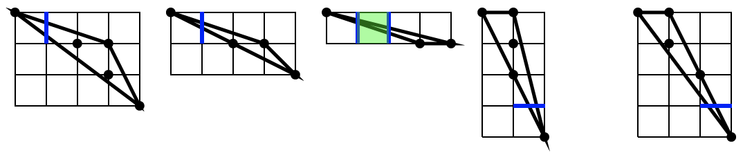
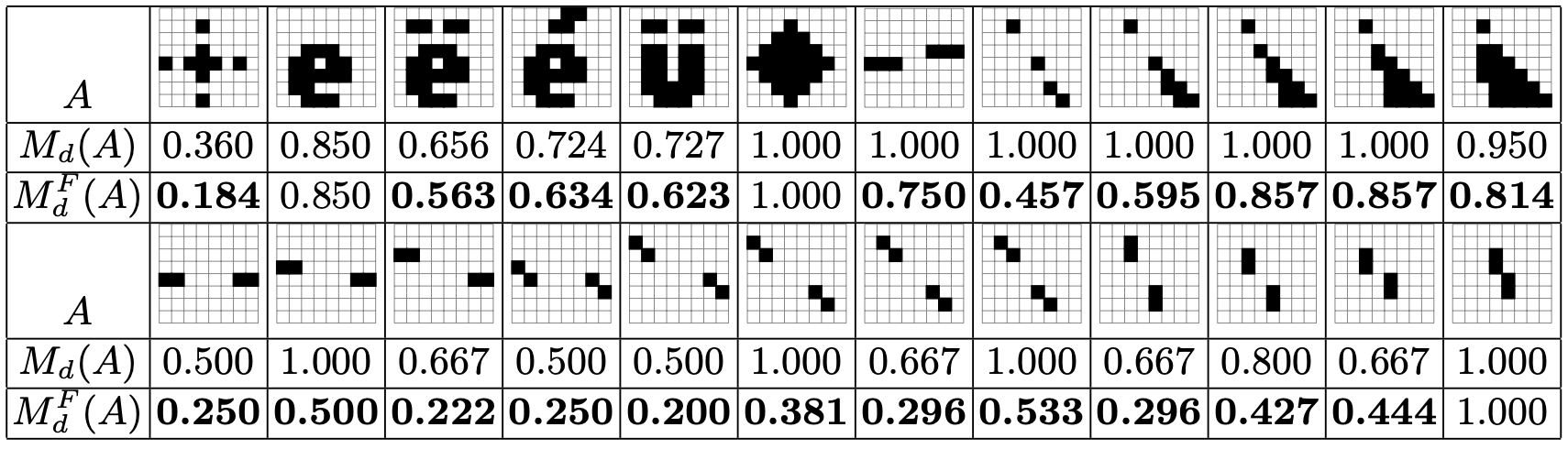
Furthermore, the recursive definition of P-convexity induces a natural measure of full convexity for digital sets. Indeed the classical d-dimensional digital convexity measure of digital set A is
\[ M_d(A):=\frac{\#(A)}{\#(\mathrm{CvxH}(A) \cap \mathbf{Z}^d)}, \]
and \( M_d(\emptyset)=1 \).
The full convexity measure \( M_d^F \) for finite digital set A is
\[ M_1^F(A) := M_1(A), \quad M_d^F(A) := M_d(A) \Pi_{k=1}^d M_{d-1}^F( \pi_k(A) )\quad\text{for}\,\, d > 1. \]
It coincides with the digital convexity measure in dimension 1, but may differ starting from dimension 2, and is always less or equal to the convexity measure.
- method PConvexity::convexityMeasure returns the convexity measure \( M_d(A) \) of the given range of digital points A,
- method PConvexity::fullConvexityMeasure returns the full convexity measure \( M_d^F(A) \) of the given range of digital points A.
The figure below illustrates the links and the differences between the two convexity measures Md and MdF on simple 2D examples. As one can see, the usual convexity measure may not detect disconnectedness and it is sensitive to specific alignments of pixels. On the contrary, full convexity is globally more stable to perturbation and is never 1 when sets are disconnected.
Best algorithm for checking full convexity
There exists multiple equivalent characterizations of full convexity. Some of them induce algorithms for checking if a digital set is indeed fully convex, but the question `‘which is the fastest way’' remains. We recap here the different characterizations for \( X \subset \mathbb{Z}^d \) being full convex, which lead to an arbitrary dimensional algorithm for checking if a given range of n points X is indeed fully convex:
discrete morphological characterization [80] [81]
X is fully convex iff \( \forall \alpha \subset \{1, \ldots, d\}, U_\alpha(X) = \mathrm{CvxH}(U_\alpha(X)) \cap \mathbb{Z}^d \),
where \( U_\alpha \) is the discrete Minkowski sum defined as \( U_\emptyset(X):= X \), and for any subset of directions \( \alpha \in \{1,\ldots,d\} \) and a direction \( i \in \alpha \), \( U_\alpha(X) := U_{\alpha \setminus \{i\}}(X) \cup \mathbf{e}_i (U_{\alpha \setminus \{i\}}(X)) \) (the latter being the unit translation of the set along direction i).
This is implemented as DigitalConvexity::isFullyConvex .
cellular characterization [54] (Lemma 13)
X is fully convex iff \( X = \mathrm{Star}(\mathrm{Cvxh}(X)) \cap \mathbb{Z}^d \).
Furthermore, Theorem 5 of [54] tells that \( \mathrm{Star}(\mathrm{CvxH}(X)) \) is directly computable from \( \mathrm{CvxH}(U_{\{1,\ldots,d\}}(X)) \), so one convex hull computation is sufficient.
This is implemented as DigitalConvexity::isFullyConvexFast .
envelope idempotence [54] (Theorem 2)
X is fully convex iff \( X = FC(X) \), where \( FC(X):=\mathrm{Extr}( \mathrm{Skel}( \mathrm{Star}( \mathrm{CvxH}( X ) ) ) ) \).
This is implemented as DigitalConvexity::envelope, but its speed is not tested here, since it is similar to the previous one
P-convexity characterization [55]
X is fully convex iff \( X \) is 0-convex, and, if \( d > 1 \), the d projections of \( X \) along each axis is P-convex (in \( \mathbb{Z}^{d-1} \)).
This is implemented as PConvexity::isPConvex .
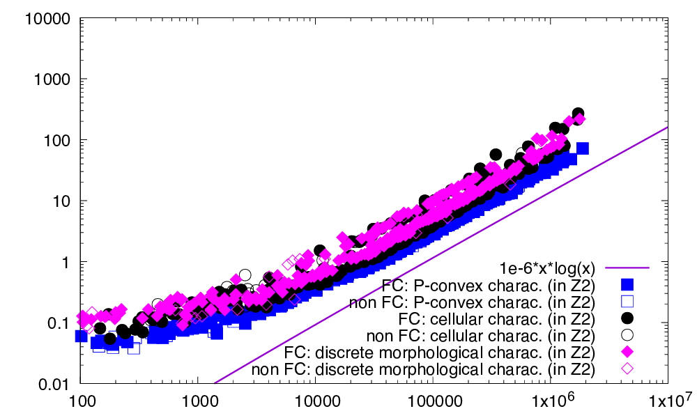
All three methods are tested for dimension 2, 3, and 4. In the first set of experiments (left of figures) we compare them on generic digital sets, which are randomly generated in a given range with a target density from \( 10\% \) to \( 90\% \). In the second set of experiments (right of figures), we limit our comparison to digital sets that are either digitally 0-convex or fully convex. We then distinguish the timings for checking full convexity depending on the output full convexity property of the input set, since it influences the computation time (typically increases it).
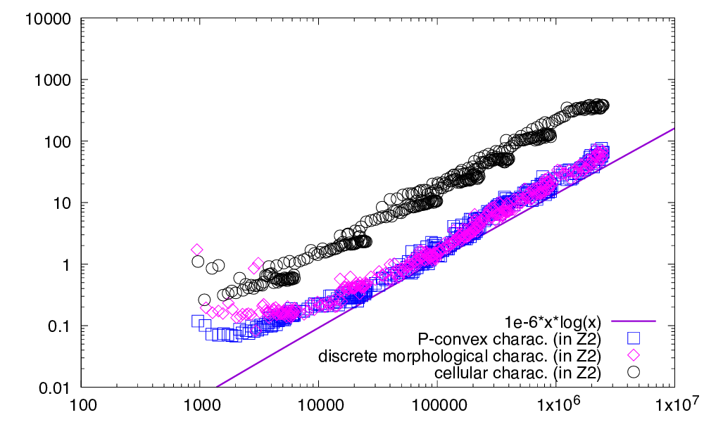
Figures below sum up the different computation times for dimension 2, 3, and 4.
| 
|
| This figure displays the respective computation times (ms) in \( \mathbb{Z}^2 \) of P-convexity (as squares), discrete morphological characterization (as diamonds) and cellular characterization (as disks), as a function of the cardinal of the digital set. Left: digital sets are randomly generated in a given range with a target point density from \( 10\% \) to \( 90\% \). Right: digital sets are randomly generated so that they are either 0-convex or fully convex. | |
| 
|
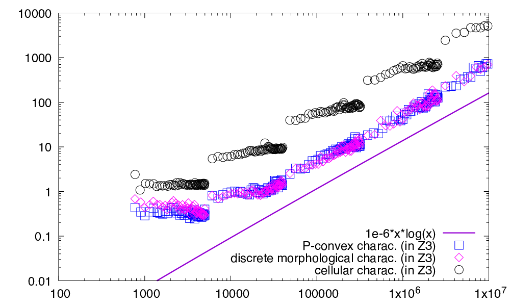
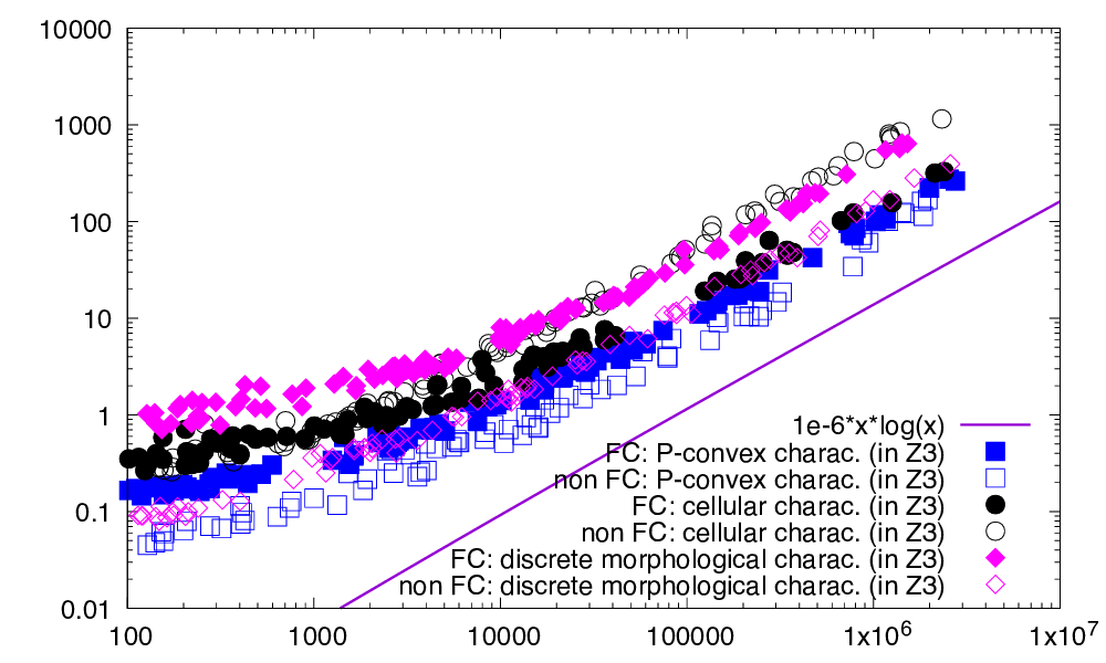
| This figure displays the respective computation times (ms) in \( \mathbb{Z}^3 \) of P-convexity (as squares), discrete morphological characterization (as diamonds) and cellular characterization (as disks), as a function of the cardinal of the digital set. Left: digital sets are randomly generated in a given range with a target point density from \( 10\% \) to \( 90\% \). Right: digital sets are randomly generated so that they are either 0-convex or fully convex. | |
| 
|
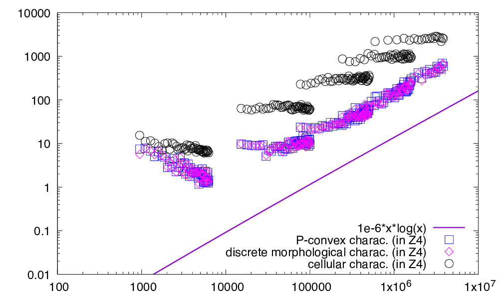
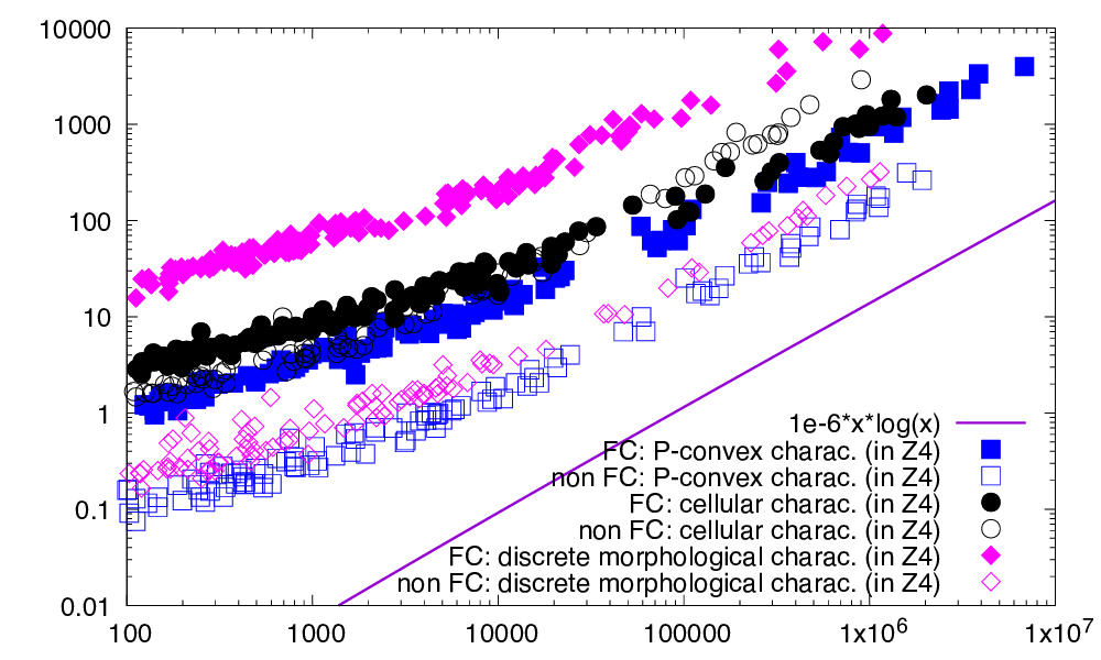
| This figure displays the respective computation times (ms) in \( \mathbb{Z}^4 \) of P-convexity (as squares), discrete morphological characterization (as diamonds) and cellular characterization (as disks), as a function of the cardinal of the digital set. Left: digital sets are randomly generated in a given range with a target point density from \( 10\% \) to \( 90\% \). Right: digital sets are randomly generated so that they are either 0-convex or fully convex. | |
All approaches follow more or less a linearithmic or subquadratic complexity \( O(n \log n) \) (tests are limited to dimension lower or equal to 4). However, we can distinguish three cases:
- if X is not even convex, both P-convexity and the discrete morphological characterization are the fastest with similar results, since both their first step involves checking 0-convexity. The cellular characterization is the slowest since it computes directly a convex hull with additional vertices.
- if X is convex but not fully convex, then the fastest method remains the P-convexity, followed by the discrete morphological characterization, and the slowest is the cellular characterization.
- if X is fully convex, then the fastest method is again the P-convexity, followed by the cellular characterization, and the slowest is the discrete morphological characterization (especially when increasing the dimension).
- Note
- Overall the P-convexity characterization (method PConvexity::isPConvex) is almost always the fastest way to check the full convexity of a given range of digital points, with speed-up from 2 to 100 times faster especially when increasing the dimension. This new characterization of full convexity is thus for now the best way to check if a digital set is fully convex.
- Warning
- One could be surprised by the last graph in 4D. Indeed we expect convex hull computations in \( O(n^2) \) in 4D. We observe here timings close to \( \Theta(n \log n) \). This is due to the fact that the digital sets we are considering are 0-convex, so "full of digital points". Convex hull computations by QuickHull are thus faster than expected since many points are "hidden" in the shape. It can also be seen on the left of this figure that timings depend more on the range of random points than on the density (e.g. see horizontal strokes of circles, corresponding to density increases), which confirms the above explanation.
Rational polytopes
You can also create bounded rational polytopes, i.e. polytopes with vertices with rational coordinates, with class BoundedRationalPolytope. You must give a common denominator for all rational coordinates.
Then the interface of BoundedRationalPolytope is almost the same as the one of BoundedLatticePolytope (see Lattice polytopes ).
The class BoundedRationalPolytope offers dilatation by an arbitrary rational, e.g. as follows
You may also check digital convexity and compute cell covers with bounded rational polytopes, exactly in the same way as with BoundedLatticePolytope.
- Note
- Big denominators increase with the same factor coefficients of half space constraints, hence the integer type should be chosen accordingly.
Further notes
The class BoundedLatticePolytope is different from the class LatticePolytope2D for the following two reasons:
- the class LatticePolytope2D is limited to 2D
- the class LatticePolytope2D is a vertex representation (or V-representation) of a polytope while the class BoundedLatticePolytope is a half-space representation (or H-representation) of a polytope.
There are no simple conversion from one to the other. Class LatticePolytope2D is optimized for cuts and lattice points enumeration, and is very specific to 2D. Class BoundedLatticePolytope is less optimized than the previous one but works in nD and provides Minkowski sum and dilation services.