Tutorial "Generated shape -> Grid curve -> Length estimation"

Table of Contents

• Implicit Gauss digitization of a Euclidean shape
• Tracking, grid curve, range
• Length estimation
• Increasing the resolution
• Length estimator comparison
• Required includes

Author(s) of this documentation:

Tristan Roussillon

In this example, we show how to test a length estimator of the contour of a generated shape, which is digitized at different resolutions.

Please have a look to shapeGridCurveEstimator.cpp to get the complete source code of this tutorial.

Implicit Gauss digitization of a Euclidean shape

Let us assume that a flower-like shape has been instanciated.
We now implicitely consider its digitization according to the Gauss scheme (set of digital points lying inside the shape).

  //implicit digitization of a shape of type Flower 
  //into a digital space of type Space
  typedef Flower2D<Z2i::Space> Flower; 
  Flower2D<Z2i::Space> flower(Z2i::Point(0,0), 20, 5, 5, 0);
  
  double h = 1; 
  GaussDigitizer<Z2i::Space,Flower> dig;  
  dig.attach( flower );
  dig.init( flower.getLowerBound()+Z2i::Vector(-1,-1),
            flower.getUpperBound()+Z2i::Vector(1,1), h ); 

Note

Similarly to the previous tutorial (Tutorial "Image -> Region -> Grid curve -> Length estimation"), the explicit construction of the digital set is not necessary.
Since the shape knows its bounding domain, it is enough to have a predicate that indicates, for each point of the domain, whether it belongs to the digital set or not. This is a useful feature when we want to digitize a shape at a high resolution.

The grid step h is given in the init method of the GaussDigitizer. The smaller the grid step, the higher the resolution is.

Tracking, grid curve, range

The extraction of the contour is performed in a cellular space (with 0-, 1-, and 2-cells), given an adjacency (0-, 1-, 2-adjacency). See Cellular grid space and topology, unoriented and oriented cells, incidence for the basic concepts of cellular topology.

  //Khalimsky space
  Z2i::KSpace ks;
  ks.init( dig.getLowerBound(), dig.getUpperBound(), true );
  //adjacency (4-connectivity)
  SurfelAdjacency<2> sAdj( true );

Since there is only one connected digital set, a fast method is used to find a first boundary element (i.e. a 1-cell between a 2-cell inside the shape and a 2-cell outside the shape). Instead of scanning the whole domain, points are randomly tested, until one point inside the shape and one point outside the shape are found. A dichotomic process is then used to retrieve the boundary element that is lying between these two points.

Note

A DGtal::InputException is raised if the method fails to find two different points.

From one boundary 1-cell, the contour is then implicitely tracked as follows:

  //searching for one boundary element
  Z2i::SCell bel = Surfaces<Z2i::KSpace>::findABel( ks, dig, 1000 );
  //tracking
  std::vector<Z2i::Point> boundaryPoints;
  Surfaces<Z2i::KSpace>
    ::track2DBoundaryPoints( boundaryPoints, ks, sAdj, dig, bel );

The GridCurve object is merely built from the retrieved contour:

  Z2i::Curve c;
  c.initFromVector( boundaryPoints );  

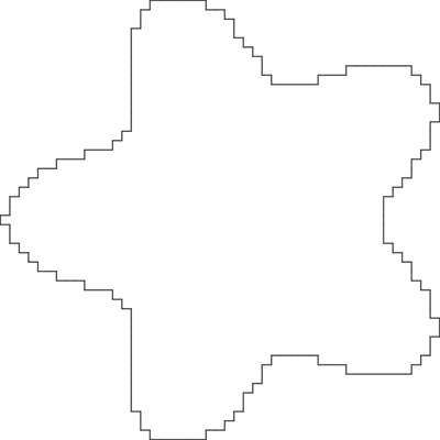
Here is a picture of the contour:

Flower (h=1)

Length estimation

The DSS approach chosen below for the length estimation requires a points range:

  //range of points
  typedef Z2i::Curve::PointsRange Range; 
  Range r = c.getPointsRange(); 

Similarly to the previous tutorial (Tutorial "Image -> Region -> Grid curve -> Length estimation"), we initialize the DSS length estimator from the points range and get the estimated length.

  //length estimation
  DSSLengthEstimator< Range::ConstCirculator > DSSlength;
  double length1 = DSSlength.eval(r.c(), r.c(), h);
  trace.info() << "Length (h=" << h << "): " << length1 << std::endl;

Note that there is a specific length estimator, which is called true length estimator, because it returns the true length (or a very close value to the true length). The only difference between the true estimator and the other ones is that the true estimator knows the shape and its parameters.

  typedef ParametricShapeArcLengthFunctor< Flower > Length;
  TrueGlobalEstimatorOnPoints< 
    Range::ConstCirculator, 
    Flower, 
    Length  >  trueLengthEstimator;
  trueLengthEstimator.attach(flower);
  // Note: Not equivalent to eval(r.c(), r.c(), h)
  double trueLength = trueLengthEstimator.eval();
  trace.info() << "ground truth: " << trueLength << std::endl;

Thanks to the true estimator, it is very easy to compare the accuracy of the estimators against a ground truth. In our example, we have:

Length (h=1): 163.646
ground truth: 165.961

Increasing the resolution

In order to have a better accuracy in the estimation, we digitize now the shape at a higher resolution, i.e. with a smaller grid step. We choose as grid step h=0.1 instead of h=1:

  //implicit digitization at higher resolution
  h = 0.1; 
  dig.init( flower.getLowerBound()+Z2i::Vector(-1,-1),
            flower.getUpperBound()+Z2i::Vector(1,1), h ); 
  //a greater domain is needed in the Khalimsky space
  ks.init( dig.getLowerBound(), dig.getUpperBound(), true );
  //searching for one boundary element
  bel = Surfaces<Z2i::KSpace>::findABel( ks, dig, 10000 );
  //tracking
  Surfaces<Z2i::KSpace>
    ::track2DBoundaryPoints( boundaryPoints, ks, sAdj, dig, bel );
  //reset grid curve and its points range
  c.initFromVector( boundaryPoints );
  Range r2 = c.getPointsRange(); 
  //estimate length
  double length2 = DSSlength.eval(r2.c(), r2.c(), h);
  trace.info() << "Length (h=" << h << "): " << length2 << std::endl;  

Here is a picture of the contour:

Flower (h=0.1)

At grid step 0.1, the estimation is better and close to the ground truth (165.961), since we get:

Length (h=0.1): 165.94

Length estimator comparison

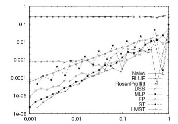
Many other length estimators are implemented (see L1LengthEstimator, BLUELocalLengthEstimator, RosenProffittLocalLengthEstimator, MLPLengthEstimator, FPLengthEstimator). You can compare them in a multiresolution framework thanks to the nice tool lengthEstimators.cpp. It provides a way of generating a given shape (whose parameters are given as arguments) at increasing resolution and list, for each resolution, the ground truth and the length estimated by all the available methods. For instance, the data of the following plot come from this tool:

Perimeter of a digitized disk of radius 10

Required includes

Here are the basic includes:

#include "DGtal/base/Common.h"
#include "DGtal/helpers/StdDefs.h"
#include "ConfigExamples.h"

In order to generate an implicite or parametric shape, you need this:

//shape and digitizer
#include "DGtal/shapes/Shapes.h"
#include "DGtal/shapes/ShapeFactory.h"
#include "DGtal/shapes/GaussDigitizer.h"

To retrieve its contour, you should add:

//tracking grid curve
#include "DGtal/topology/helpers/Surfaces.h"
#include "DGtal/geometry/curves/GridCurve.h"

And finally the length estimation requires:

//length estimation knowing the shape
#include "DGtal/geometry/curves/estimation/TrueGlobalEstimatorOnPoints.h"
#include "DGtal/geometry/curves/estimation/ParametricShapeArcLengthFunctor.h"
//length estimation based on a DSS segmentation
#include "DGtal/geometry/curves/estimation/DSSLengthEstimator.h"