Loading...
Searching...
No Matches
Estimator Tools
2dLocalEstimators
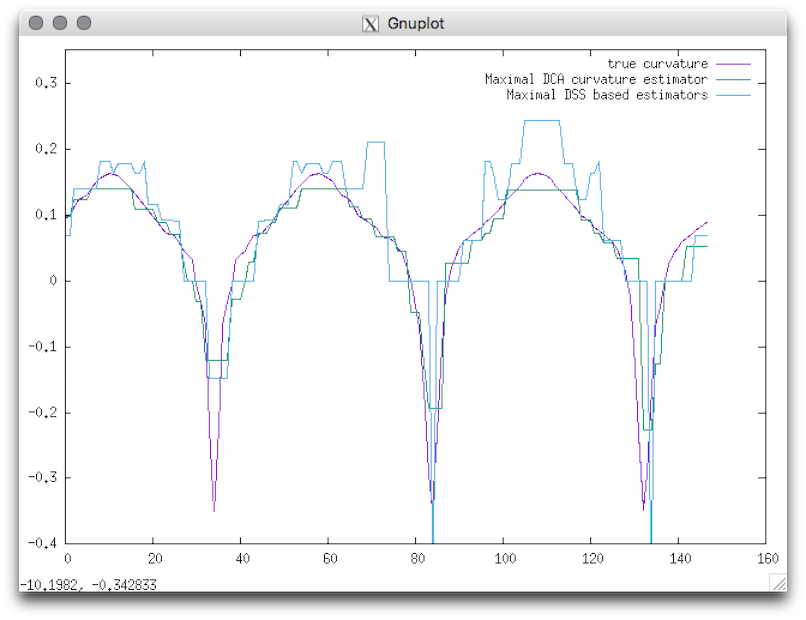
Usage: 2dlocalEstimators –output <output> –shape <shapeName> [required parameters] –estimators <binaryWord> –properties <binaryWord>Below are the different available families of estimators:Example: With this tool you can easely compare several estimator with the real value: You can display the result by using gnuplot:You should obtain such a graph:
- True estimators
- Maximal DSS based estimators
- Maximal DCA based estimators
- Binomial convolver based estimators
- Integral Invariants based estimators
- Tangent
- Curvature
-h,--help Print this help message and exit
-l,--list List all available shapes
-o,--output TEXT REQUIRED Output
-s,--shape TEXT REQUIRED Shape name
-R,--radius FLOAT Radius of the shape
-K,--kernelradius FLOAT=2.35162e-314 Radius of the convolution kernel (Integral invariants estimators)
--alpha FLOAT=0.333333 Alpha parameter for Integral Invariant computation
-A,--axis1 FLOAT Half big axis of the shape (ellipse)
-a,--axis2 FLOAT Half small axis of the shape (ellipse)
-r,--smallradius FLOAT=5 Small radius of the shape
-v,--varsmallradius FLOAT=5 Variable small radius of the shape
-k UINT=3 Number of branches or corners the shape (default 3)
--phi FLOAT=0 Phase of the shape (in radian)
-w,--width FLOAT=10 Width of the shape
-p,--power FLOAT=2 Power of the metric
-x,--center_x FLOAT=0 x-coordinate of the shape center
-y,--center_y FLOAT=0 y-coordinate of the shape center
-g,--gridstep FLOAT=1 Gridstep for the digitization
-n,--noise FLOAT=0 Level of noise to perturb the shape
--properties TEXT=11 the i-th property is disabled iff there is a 0 at position i
-e,--estimators TEXT=1000 the i-th estimator is disabled iff there is a 0 at position i
-E,--exportShape TEXT Exports the contour of the source shape as a sequence of discrete points (.sdp)
--lambda BOOLEAN=0 Use the shape to get a better approximation of the surface (optional)
$ 2dlocalEstimators --output curvature --shape flower --radius 15 -v 5 --gridstep 1 --estimators 11100 --properties 01
$ gnuplot
gnuplot> plot [][-0.4:0.35] 'curvature_True_curvature.dat' w lines title "true curvature" , 'curvature_MDCA_curvature.dat' w lines title "Maximal DCA curvature estimator", 'curvature_MDSSl_curvature.dat' w lines title "Maximal DSS based estimators"
Resulting visualization.
- See also
- 2dLocalEstimators.cpp
3dCurveTangentEstimator
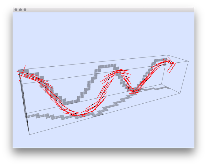
Usage: ./estimators/3dCurveTangentEstimator [options] –input <filename>This program estimates the tangent vector to a set of 3D integer points, which are supposed to approximate a 3D curve. This set of points is given as a list of points in file <input>. The tangent estimator uses either the digital Voronoi Covariance Measure (VCM) or the 3D lambda-Maximal Segment Tangent (L-MST). This program can also displays the curve and tangent estimations, and it can also extract maximal digital straight segments (2D and 3D).
Example: This command line show an example of tangent estimation with the VCM estimator.
You should obtain such a result:
- Note
- It is not compulsory for the points to be ordered in sequence, except if you wish to compute maximal digital straight segments. In this case, you can select the connectivity of your curve between 6 (standard) or 26 (naive).
Allowed options are :
Positionals:
1 TEXT:FILE REQUIRED the name of the text file containing the list of 3D points: (x y z) per line.
Options:
-h,--help Print this help message and exit
-i,--input TEXT:FILE REQUIRED the name of the text file containing the list of 3D points: (x y z) per line.
-V,--view TEXT=OFF toggles display ON/OFF
-b,--box INT=0 specifies the tightness of the bounding box around the curve with a given integer displacement <arg> to enlarge it (0 is tight)
-v,--viewBox TEXT:{WIRED,COLORED}=WIRED
displays the bounding box, <arg>=WIRED means that only edges are displayed, <arg>=COLORED adds colors for planes (XY is red, XZ green, YZ, blue).
-T,--connectivity TEXT:{6,26}=6 specifies whether it is a 6-connected curve or a 26-connected curve: arg=6 | 26.
-C,--curve3d displays the 3D curve
-c,--curve2d displays the 2D projections of the 3D curve on the bounding box
-3,--cover3d displays the 3D tangential cover of the curve
-2,--cover2d displays the 2D projections of the 3D tangential cover of the curve
-t,--tangent displays the tangents to the curve.
-n,--nbColors UINT=3 sets the number of successive colors used for displaying 2d and 3d maximal segments (default is 3: red, green, blue)
-R,--big-radius FLOAT=10 the radius parameter R in the VCM estimator.
-r,--small-radius FLOAT=3 the radius parameter r in the VCM estimator.
-m,--method TEXT:{VCM,L-MST}=VCM the method of tangent computation: VCM (default), L-MST.
-a,--axes TEXT:{ON,OFF}=OFF show main axes - prints list of axes for each point and color points color = (if X => 255, if Y => 255, if Z => 255)
-o,--output TEXT=3d-curve-tangent-estimations
the basename of the output text file which will contain points and tangent vectors: (x y z tx ty tz) per line
3dCurveTangentEstimator ${DGtal}/examples/samples/sinus.dat -V ON -c -R 20 -r 3 -T 6
Definition ATu0v1.h:57
Resulting tangent vectors (red) obtained with the VCM estimator.
- See also
- 3dCurveTangentEstimator.cpp
3dLocalEstimators
Usage: 3dLocalEstimators [options] –shape <shape> –h <h> –radius <radius> –estimators <binaryWord> –output <output>Below are the different available families of estimators:Example: The following example will estimate the curvature of an implicit cone shape and will produce six resulting files (toto_II_gaussian.dat,toto_II_mean.dat, toto_MongeJetFitting_gaussian.dat, toto_MongeJetFitting_mean.dat, toto_True_gaussian.dat, toto_True_mean.dat)
- Integral Invariant Mean
- Integral Invariant Gaussian
- Monge Jet Fitting Mean
- Monge Jet Fitting Gaussian
-h,--help Print this help message and exit
-s,--shape TEXT REQUIRED Shape
-o,--output TEXT=result.dat REQUIRED Output file
-r,--radius FLOAT REQUIRED Kernel radius for IntegralInvariant
--alpha FLOAT=0.333333 Alpha parameter for Integral Invariant computation
--h FLOAT REQUIRED Grid step
-a,--minAABB FLOAT=-10 Min value of the AABB bounding box (domain)
-A,--maxAABB FLOAT=10 Max value of the AABB bounding box (domain)
-n,--noise FLOAT=0 Level of noise to perturb the shape
-l,--lambda Use the shape to get a better approximation of the surface (optional)
--properties TEXT=110 the i-th property is disabled iff there is a 0 at position i
-e,--estimators TEXT=110 the i-th estimator is disabled iff there is a 0 at position i
./estimators/3dlocalEstimators --shape "z^2-x^2-y^2" --output result --h 0.4 --radius 1.0
You can check other example of implicit shapes like the followinf:
- whitney : x^2-y*z^2
- 4lines : x*y*(y-x)*(y-z*x)
- cone : z^2-x^2-y^2
- simonU : x^2-z*y^2+x^4+y^4
- cayley3 : 4*(x^2 + y^2 + z^2) + 16*x*y*z - 1
- crixxi : -0.9*(y^2+z^2-1)^2-(x^2+y^2-1)^3
curvatureBC
Usage: curvatureBC [options] –input <fileName>Allowed options are :
Example: We consider as input shape the freeman chain of the DGtal/examples/sample directory. The contour can be displayed with displayContours : The curvature can be computed as follows: You should obtain such a result:
Positionals:
1 TEXT:FILE REQUIRED Input FreemanChain file name
Options:
-h,--help Print this help message and exit
-i,--input TEXT:FILE REQUIRED Input FreemanChain file name
--GridStep FLOAT=1 Grid step
$ displayContours $DGtal/examples/samples/contourS.fc contourS.png --drawPointOfIndex 0
$ curvatureBC $DGtal/examples/samples/contourS.fc > curvatureBC.dat
$ gnuplot
gnuplot> plot 'curvatureBC.dat' w lines title "curvature with Binomial Convolution estimator"
| contour | curvature |
|---|---|
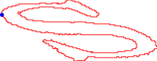 | 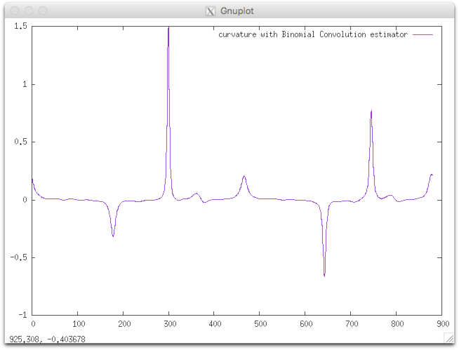 |
| CCW oriented (index 0=blue pt) | resulting curvature |
- See also
- curvatureBC.cpp
curvatureMCMS
Usage: curvatureMCMS [options] –input <fileName>Allowed options are :
Example: We consider as input shape the freeman chain of the DGtal/examples/sample directory. The contour can be displayed with displayContours : The curvature can be computed as follows: You should obtain such a result:
Positionals:
1 TEXT:FILE REQUIRED Input FreemanChain file name
Options:
-h,--help Print this help message and exit
-i,--input TEXT:FILE REQUIRED Input FreemanChain file name
--GridStep FLOAT=1 Grid step
$ displayContours $DGtal/examples/samples/contourS.fc contourS.png --drawPointOfIndex 0
$ curvatureMCMS $DGtal/examples/samples/contourS.fc > curvatureMCMS.dat
$ gnuplot
gnuplot> plot 'curvatureMCMS.dat' w lines title "curvature using length of most centered segment computers estimator"
| contour | curvature |
|---|---|
| | 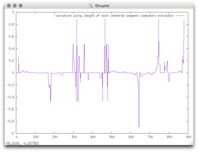 |
| CCW oriented (index 0=blue pt) | resulting curvature |
- See also
- curvatureMCMS.cpp
curvatureScaleSpaceBCC
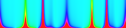
The x axis is associated to the contour point and the y axis to the scale. The colors represent the curvature values included between the cutoff values (set to 10 by default).Usage: curvatureScaleSpaceBCC –input <filename> –output <filename>Allowed options are :
Example: You should obtain such a result:
Positionals:
1 TEXT:FILE REQUIRED Input FreemanChain file name
2 TEXT REQUIRED Set the output name
Options:
-h,--help Print this help message and exit
-i,--input TEXT:FILE REQUIRED Input FreemanChain file name
-o,--output TEXT REQUIRED Set the output name
--gridStepInit FLOAT=1 Grid step initial
--gridStepIncrement FLOAT=1 Grid step increment
--gridStepFinal FLOAT=1 Grid step final
-c,--curvatureCutOff FLOAT=10 set the curvature limits to better display
$ curvatureScaleSpaceBCC ${DGtal}/examples/samples/contourS.fc --gridStepInit 0.001 --gridStepIncrement 0.0005 --gridStepFinal 0.1 -o cssResu.ppm
Resulting visualization.
- See also
- curvatureScaleSpaceBCC.cpp
eulerCharacteristic
The vol file is first binarized using interval [m,M[ thresholds and the Eucler characteristic is given from the cubical complex.Usage: eulerCharacteristic –input <volFileName> -m <minlevel> -M <maxlevel>Allowed options are :
Example: You should obtain such a result:
Positionals:
1 TEXT:FILE REQUIRED Input vol file.
Options:
-h,--help Print this help message and exit
-i,--input TEXT:FILE REQUIRED Input vol file.
-m,--thresholdMin INT=0 threshold min (excluded) to define binary shape (default 0)
-M,--thresholdMax INT=255 threshold max (included) to define binary shape (default 255)
eulerCharacteristic -i $DGtal/examples/samples/cat10.vol -m 0
Got 72479 cells
Got 10128 pointels 28196 linels  26112 surfels and 8043  bells
Volumetric Euler Characteristic = 1
- See also
- eulerCharacteristic.cpp
generic3dNormalEstimators
Usage: ./estimators/generic3dNormalEstimators -p <polynomial> [options]Computes a normal vector field over a digitized 3D implicit surface for several estimators (II|VCM|Trivial|True), specified with -e. You may add Kanungo noise with option -N. These estimators are compared with ground truth. You may then: 1) visualize the normals or the angle deviations with -V (if DGTAL_WITH_POLYSCOPE_VIEWER is enabled), 2) outputs them as a list of cells/estimations with -n, 3) outputs them as a ImaGene file with -O, 4) outputs them as a NOFF file with -O, 5) computes estimation statistics with option -S.Allowed options are :Example of implicit surface (specified by -p):
It is also possible to visualize the resulting normals:
-h,--help Print this help message and exit
-p,--polynomial TEXT REQUIRED the implicit polynomial whose zero-level defines the shape of interest.
-N,--noise FLOAT=0 the Kanungo noise level l=arg, with l^d the probability that a point at distance d is flipped inside/outside.
-a,--minAABB FLOAT=-10 the min value of the AABB bounding box (domain)
-A,--maxAABB FLOAT=10 the max value of the AABB bounding box (domain)
-g,--gridstep FLOAT=1 the gridstep that defines the digitization (often called h).
-e,--estimator TEXT:{True,VCM,II,Trivial}=True
the chosen normal estimator: True | VCM | II | Trivial
-R,--R-radius FLOAT=5 the constant for parameter R in R(h)=R h^alpha (VCM).
-r,--r-radius FLOAT=3 the constant for parameter r in r(h)=r h^alpha (VCM,II,Trivial).
-k,--kernel TEXT=hat the function chi_r, either hat or ball.
--alpha FLOAT=0 the parameter alpha in r(h)=r h^alpha (VCM).
-t,--trivial-radius FLOAT=3 the parameter t defining the radius for the Trivial estimator. Also used for reorienting the VCM.
-E,--embedding INT=0 the surfel -> point embedding for VCM estimator: 0: Pointels, 1: InnerSpel, 2: OuterSpel.
-o,--output TEXT=output the output basename. All generated files will have the form <arg>-*, for instance <arg>-angle-deviation-<gridstep>.txt, <arg>-normals-<gridstep>.txt, <arg>-cells-<gridstep>.txt, <arg>-noff-<gridstep>.off.
-S,--angle-deviation-stats computes angle deviation error and outputs them in file <basename>-angle-deviation-<gridstep>.txt, as specified by -o <basename>.
-x,--export TEXT=None exports surfel normals which can be viewed with ImaGene tool 'viewSetOfSurfels' in file <basename>-cells-<gridstep>.txt, as specified by -o <basename>. Parameter <arg> is None|Normals|AngleDeviation. The color depends on the angle deviation in degree: 0 metallic blue, 5 light cyan, 10 light green, 15 light yellow, 20 yellow, 25 orange, 30 red, 35, dark red, 40- grey
-n,--normals outputs every surfel, its estimated normal, and the ground truth normal in file <basename>-normals-<gridstep>.txt, as specified by -o <basename>.
-O,--noff exports the digital surface with normals as NOFF file <basename>-noff-<gridstep>.off, as specified by -o <basename>..
-V,--view TEXT view the digital surface with normals. Parameter <arg> is None|Normals|AngleDeviation. The color depends on the angle deviation in degree: 0 metallic blue, 5 light cyan, 10 light green, 15 light yellow, 20 yellow, 25 orange, 30 red, 35, dark red, 40- grey.
- ellipse : 90-3*x^2-2*y^2-z^2
- torus : -1*(x^2+y^2+z^2+6*6-2*2)^2+4*6*6*(x^2+y^2)
- rcube : 6561-x^4-y^4-z^4
- goursat : 8-0.03*x^4-0.03*y^4-0.03*z^4+2*x^2+2*y^2+2*z^2
- distel : 10000-(x^2+y^2+z^2+1000*(x^2+y^2)*(x^2+z^2)*(y^2+z^2))
- leopold : 100-(x^2*y^2*z^2+4*x^2+4*y^2+3*z^2)
- diabolo : x^2-(y^2+z^2)^2
- heart : -1*(x^2+2.25*y^2+z^2-1)^3+x^2*z^3+0.1125*y^2*z^3
- crixxi : -0.9*(y^2+z^2-1)^2-(x^2+y^2-1)^3
- True : supposed to be the ground truth for computations. Of course, it is only approximations.
- VCM : normal estimator by digital Voronoi Covariance Matrix. Radii parameters are given by -R, -r.
- II : normal estimator by Integral Invariants. Radius parameter is given by -r.
- Trivial : the normal obtained by average trivial surfel normals in a ball neighborhood. Radius parameter is given by -r.
- Note
- :
- This is a normal direction evaluator more than a normal vector evaluator. Orientations of normals are deduced from ground truth. This is due to the fact that II and VCM only estimates normal directions.
- This tool only analyses one surface component, and one that contains at least as many surfels as the width of the digital bounding box. This is required when analysing noisy data, where a lot of the small components are spurious. The drawback is that you cannot analyse the normals on a surface with several components.
Example:
- Example of normal comparisons: You can estimate the normal vectors and compare the error with the true normals (option -V AngleDeviation): You should obtain such a result:# apply the Integral Invariant estimator (options -e II -r 8 ):$ generic3dNormalEstimators -p "10000-(x^2+y^2+z^2+1000*(x^2+y^2)*(x^2+z^2)*(y^2+z^2))" -a -10 -A 10 -e II -r 8 -V AngleDeviation -g 0.05# apply the Voronoi Covariance Measure based estimator (options -e VCM -r 8 ):$ generic3dNormalEstimators -p "10000-(x^2+y^2+z^2+1000*(x^2+y^2)*(x^2+z^2)*(y^2+z^2))" -a -10 -A 10 -e VCM -R 20 -r 8 -V AngleDeviation -g 0.05
type visualization digital surface 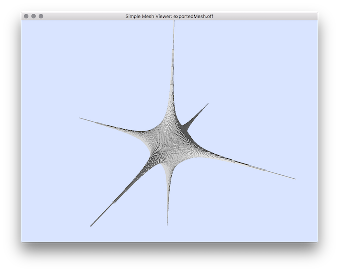
VCM angle-deviation 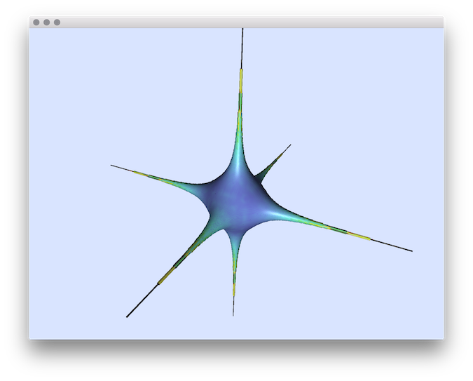
II angle-deviation 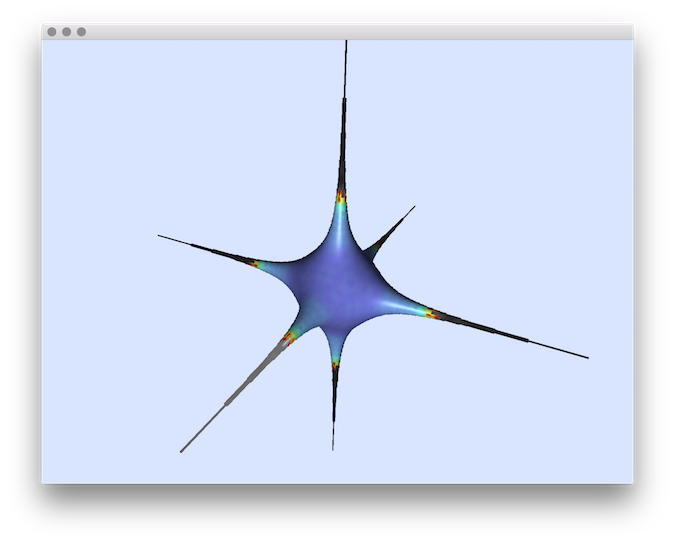
- Example of normal comparisons visualization with noise add: This tool allows to add some noise on initial shape (option -N) before estimating and comparing the normals: # apply the Integral Invariant estimator (options -e II -r 6 ):generic3dNormalEstimators -p "100-(x^2*y^2*z^2+4*x^2+4*y^2+3*z^2)" -a -10 -A 10 -e II -r 6 -V AngleDeviation -g 0.1 -N 0.3# apply the Voronoi Covariance Measure based estimator (options -e VCM -r 8 ):generic3dNormalEstimators -p "100-(x^2*y^2*z^2+4*x^2+4*y^2+3*z^2)" -a -10 -A 10 -e VCM -R 10 -r 5 -V AngleDeviation -g 0.1 -N 0.3
| type | visualization |
|---|---|
| digital surface | 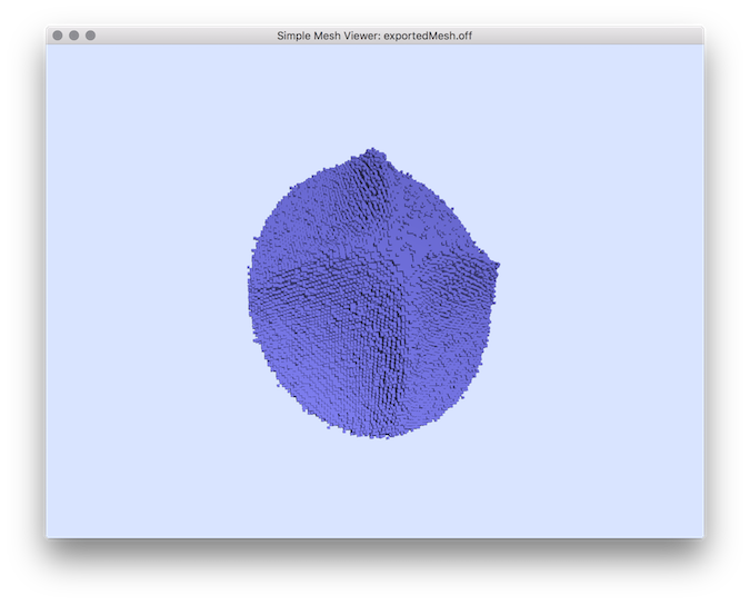 |
| VCM estimator |  |
| II estimator |  |
# display the II normals:
generic3dNormalEstimators -p "100-(x^2*y^2*z^2+4*x^2+4*y^2+3*z^2)" -a -10 -A 10 -e II -r 8 -V Normals -g 0.3
You should obtain such a result:
| type | visualization |
|---|---|
| II estimator | 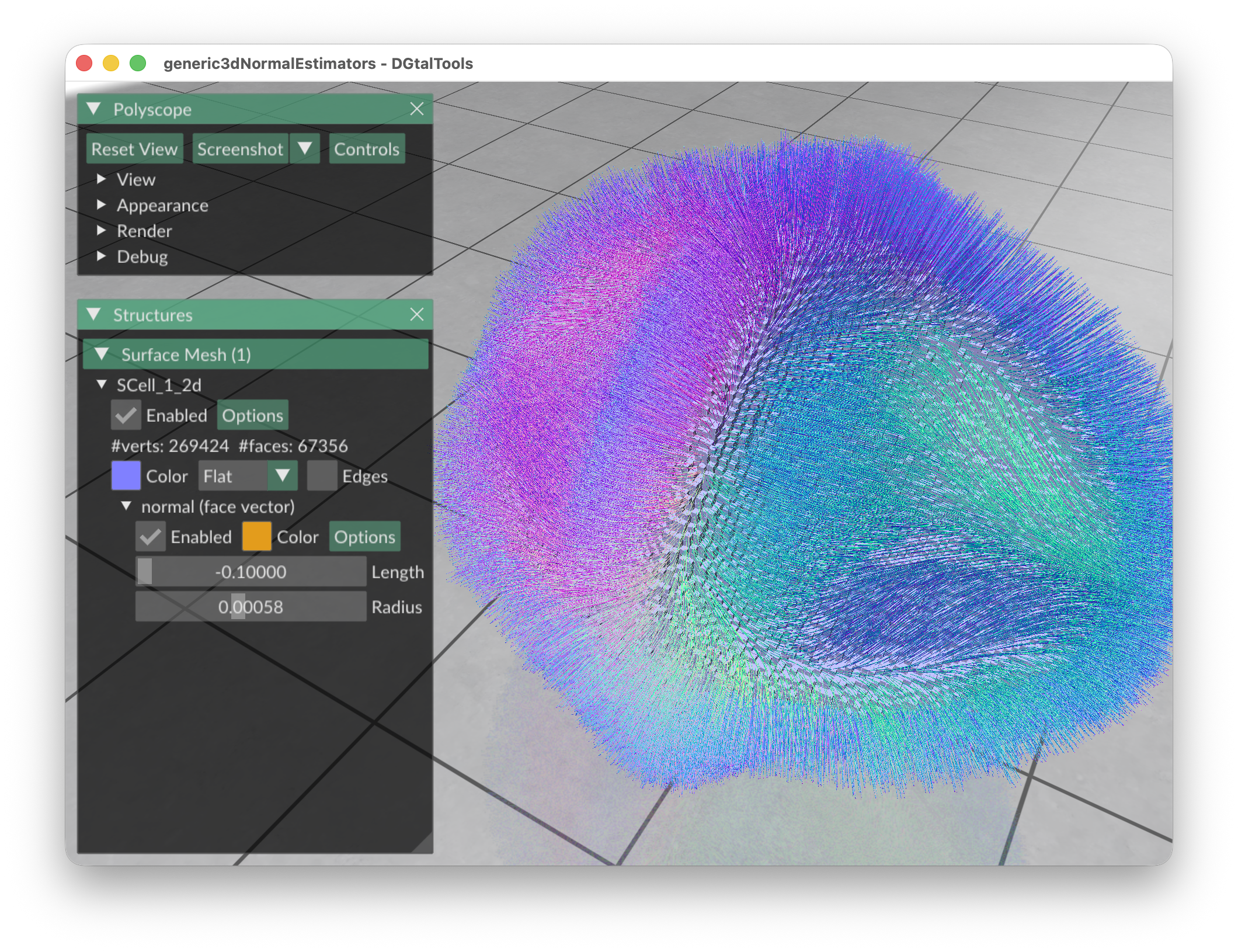 |
- See also
- generic3dNormalEstimators.cpp
lengthEstimators
It will output length estimations (and timings) using several algorithms for decreasing grid steps.Usage: LengthEstimators [options] –shape <shapeName>Allowed options are : The list of 2D shape are : -ball Ball for the Euclidean metric. Required parameter(s): –radius [-R]You can display using gnuplot:You should obtain such a result:
-h,--help Print this help message and exit
-l,--list List all available shapes
-s,--shape TEXT Shape name
-R,--radius FLOAT Radius of the shape
-A,--axis1 FLOAT Half big axis of the shape (ellipse)
-a,--axis2 FLOAT Half small axis of the shape (ellipse)
-r,--smallradius FLOAT=5 Small radius of the shape (default 5)
-v,--varsmallradius FLOAT=5 Variable small radius of the shape (default 5)
-k UINT=3 Number of branches or corners the shape (default 3)
--phi FLOAT=0 Phase of the shape (in radian, default 0.0)
-w,--width FLOAT=10 Width of the shape (default 10.0)
-p,--power FLOAT=2 Power of the metric (default 2.0)
--hMin FLOAT=0.0001 Minimum value for the grid step h (double, default 0.0001)
--steps INT=32 Number of multigrid steps between 1 and hMin (integer, default 32)
- square square (no signature). Required parameter(s): –width [-w]
- lpball Ball for the l_power metric (no signature). Required parameter(s): –radius [-R], –power [-p]
- flower Flower with k petals. Required parameter(s): –radius [-R], –varsmallradius [-v], –k [-k], –phi
- ngon Regular k-gon. Required parameter(s): –radius [-R], –k [-k], –phi
- accflower Accelerated Flower with k petals. Required parameter(s): –radius [-R], –varsmallradius [-v], –k [-k], –phi
- ellipse Ellipse. Required parameter(s): –axis1 [-A], –axis2 [-a], –phi
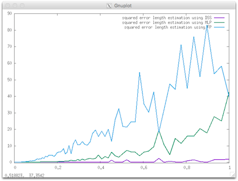
$ lengthEstimators -s flower -k 5 -R 20 -r 5 --steps 256 > length.dat
$ gnuplot
gnuplot> plot [0:][-0.5: 90] 'length.dat' using 1:(($7-$3)*($7-$3)) w l title "squared error length estimation using DSS", 'length.dat' using 1:(($8-$3)*($8-$3)) w l title "squared error length estimation using MLP", 'length.dat' using 1:(($9-$3)*($9-$3)) w l title "squared error length estimation using FP" linewidth 2
Resulting visualization.
- See also
- lengthEstimators.cpp
statisticsEstimators
Usage: statisticsEstimators –file1 <file1> –column1 <column1> –file2 <file2> –column2 <column2> –output <output>Allowed options are :
Example: This tool can be used in association to other estimator with for instance the 2dLocalEstimators which gives as output a file containing the curvature:Then you can use this tool as follows: The resulting file result.dat should contains:
Positionals:
1 TEXT:FILE REQUIRED File 1.
2 TEXT:FILE REQUIRED File 2.
Options:
-h,--help Print this help message and exit
-f,--file1 TEXT:FILE REQUIRED File 1.
-F,--file2 TEXT:FILE REQUIRED File 2.
-c,--column1 UINT REQUIRED Column of file 1
-C,--column2 UINT REQUIRED Column of file 2
-o,--output TEXT REQUIRED Output file
-m,--monge BOOLEAN=0 Is from Monge mean computation (optional, default false)
./estimators/2dlocalEstimators --output curvature --shape flower --radius 15 -v 5 --gridstep 1 --estimators 11100 --properties 01
./estimators/statisticsEstimators --file1 curvature_True_curvature.dat --column1 0 --file2 curvature_II_curvature.dat --column2 0 -o result.dat
# h | L1 Mean Error | L2 Mean Error | Loo Mean Error
1 0.0844106 0.0108399 0.519307
- See also
- statisticsEstimators.cpp
tangentBC
Usage: tangentBC [options] –input <fileName>Allowed options are :
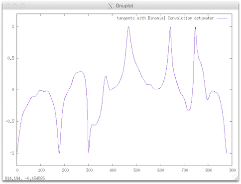
The tangents can be computed as follows: You should obtain such a result:
Positionals:
1 TEXT:FILE REQUIRED input file name: FreemanChain (.fc) or a sequence of discrete points (.sdp).
Options:
-h,--help Print this help message and exit
-i,--input TEXT:FILE REQUIRED input file name: FreemanChain (.fc) or a sequence of discrete points (.sdp).
--GridStep FLOAT=1 Grid step (default 1.0)
- Note
- The file may contain several freeman chains.
Example: We consider as input shape the freeman chain of the DGtal/examples/sample directory. The contour can be displayed with displayContours :
$ displayContours $DGtal/examples/samples/contourS.fc contourS.png --drawPointOfIndex 0
$ tangentBC $DGtal/examples/samples/contourS.fc > tangentsBC.dat
$ gnuplot
gnuplot> plot [] [-1.2:1.2]'tangentsBC.dat' using 1:3 w lines title "tangents with Binomial Convolution estimator"
| contour | curvature |
|---|---|
| |  |
| CCW oriented (index 0=blue pt) | resulting tangent (angle) |
- See also
- tangentBC.cpp
vol2normalField
It will output the embedded vector field (Gaussian convolution on elementary normal vectors) an OFF file, and a TXT normal vector file (theta, phi in degree).Usage: vol2normalField[options] –input <volFileName> –o <outputFileName>Allowed options are :
Example: We consider the generation of normal vector field from the Iso-level 40 and export the vectors with a norm = -3 (negative value to invert the normal direction).You can use the too meshViewer to display the resulting vector field with the Iso-level surface: You should obtain such a result:

Positionals:
1 TEXT:FILE REQUIRED Input vol file.
2 TEXT REQUIRED Output file.
Options:
-h,--help Print this help message and exit
-i,--input TEXT:FILE REQUIRED Input vol file.
-o,--output TEXT REQUIRED Output file.
-l,--level UINT=0 Iso-level for the surface construction (default 0).
-s,--sigma FLOAT=5 Sigma parameter of the Gaussian kernel (default 5.0).
--exportOriginAndExtremity exports the origin and extremity of the vector fields when exporting the vector field in TXT format (useful to be displayed in other viewer like meshViewer).
-N,--vectorsNorm FLOAT=1 set the norm of the exported vectors in TXT format (when the extremity points are exported with --exportOriginAndExtremity). By using a negative value you will invert the direction of the vectors (default 1.0).
-n,--neighborhood UINT=10 Size of the neighborhood for the convolution (distance on surfel graph, default 10).
(distance on surfel graph).
$ vol2normalField -i $DGtal/examples/samples/lobster.vol -o lobTreshold40 -l 40 --exportOriginAndExtremity -N -3
$ meshViewer lobTreshold40.off -f lobTreshold40.txt --vectorFieldIndex 2 3 4 5 6 7 -n
Resulting vector field visualization.
- See also
- vol2normalField.cpp
volSurfaceRegularization
This is done by minimizing a quadratic energy function as decribed in ??. The variational formulation regularizes the position while aligning the regularized quads with an input normal vector field. In this tool, the input normal vector field can be either specified in the CSV input file, or computed using Integral Invariant (and -r option).Usage: volSurfaceRegularization -input <volFileName> -o <regularizedcomplex.obj>Allowed options are :
Example: You should obtain such a result:
Positionals:
1 TEXT REQUIRED input vol filename for image shape (object voxels have values > 0) or input cvs filename for surfels and normals
1 TEXT REQUIRED output regularized obj
Options:
-h,--help Print this help message and exit
-i,--image-filename TEXT REQUIRED input vol filename for image shape (object voxels have values > 0) or input cvs filename for surfels and normals
-o,--regularized-obj-filename TEXT REQUIRED
output regularized obj
-n,--cubical-obj-filename TEXT output cubical obj
-k,--shape-noise FLOAT=0 noise shape parameter
[Option Group: Normal field estimator options]
Options:
-r,--normal-radius FLOAT=4 radius of normal estimator
[Option Group: Surface approximation options]
Options:
-p,--regularization-position FLOAT=0.001
vertex position regularization coeff
-c,--regularization-center FLOAT=0.01 face center regularization coeff
-a,--align FLOAT=1 normal alignment coeff
-f,--fairness FLOAT=0 face fairness coeff
-b,--barycenter FLOAT=0.1 barycenter fairness coeff
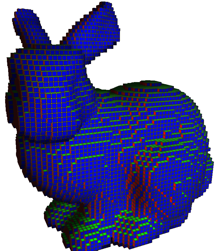
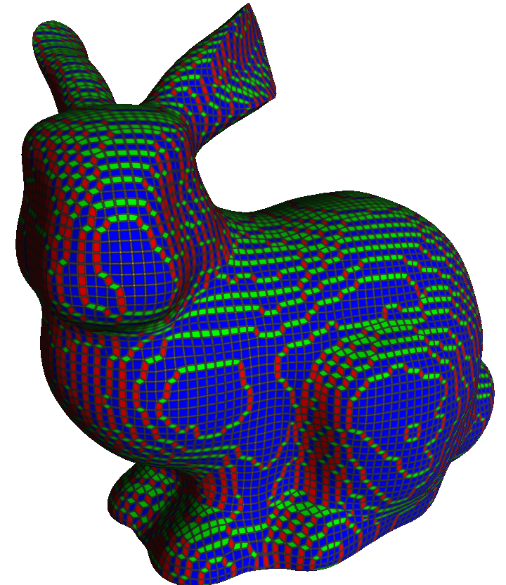
$ volSurfaceRegularization -i bunny.vol -o bunny_smooth.obj
Input cubical complex.
Smooth quadrangulated complex.
- See also
- volSurfaceRegularization.cpp